The coupled damage–plasticity material model combines damage mechanics with a plasticity model to describe important characteristics of the mechanical response and failure of concrete and similar materials subjected to multiaxial and cyclic loading conditions. Specifically, it implements the constitutive model for concrete suggested in Ref. 29 and Ref. 30.

The general constitutive equations for the coupled damage–plasticity model uses the concept of the damaged stress tensor σd and the undamaged stress tensor σun. The former is used in the weak formulation while the latter describe the behavior of the intact material.

where σun is split into a positive and negative part by a spectral decomposition in order to account for the anisotropic behavior of concrete in tension and compression. For the same reason, two damage variables introduced: the tensile damage variable dt and the compressive damage variable dc. These variables introduce a weakening of the material’s stiffness, and varies from 0 for an undamaged state to 1 for a fully damaged state. Their definitions are described in Damage Model.

The behavior of the intact material is commonly described by a linear elastic material such that Hooke’s law relates σun to the elastic strain tensor

where, C is the fourth order elasticity tensor, “:” stands for the double-dot tensor product (or double contraction). The elastic strain εel is the difference between the total strain ε and inelastic strains εinel. The coupled damage–plasticity model always adds a plastic strain tensor εpl to εinel, but other contributions such as thermal strains can also be considered. There may also be an external stress contribution σex, with contributions from initial, viscoelastic, or other inelastic stresses.

The evolution of the plastic strains are based on the undamaged stress and thus independent of damage. A flow plasticity model with isotropic hardening is used that introduces a yield function Fp, a plastic potential Qp, a scalar hardening variable κp, and the plastic multiplier λp. The model can be summarized by the following evolution equations for the plastic strain and the hardening variable

The yield function used is a generalization of The Willam–Warnke Criterion written as a function of the Haigh–Westergaard coordinates in the space of the undamaged stress tensor (ξun, run, θun), as described in Invariants of the Stress Tensor, and κp. It is defined as

where qh1 and qh2 are dimensionless hardening functions, and σcs is the uniaxial compressive strength. The friction parameter

where σts is the uniaxial tensile strength and e is the eccentricity parameter. The meridians of the corresponding yield surface Fp are parabolic, while the deviatoric sections are triangular at low confinement but changes toward a circular shape at high confinement. The shape of the deviatoric section is given by a dimensionless function of the Lode angle θun

As suggested in Ref. 29 and Ref. 30, the eccentricity is in COMSOL Multiphysics computed as

where σbc is the biaxial compressive strength.

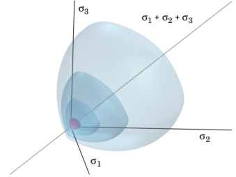
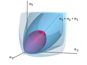
A graphical representation of yield surface Fp = 0 in the undamaged principal stress space and how evolves during hardening is shown in Figure 3-23 and Figure 3-24.

The plastic flow is determined by a non-associative flow rule; an associative flow rule typically leads to an overestimation of the strength of concrete due to an unrealistically large volume expansion during plastic flow. Here the plastic potential is a simplified version of the yield function in that it is independent of θun, and is given as

where Aq(κp) and Bq(κp) are auxiliary functions derived from assumptions on the plastic flow in the post-peak regime in uniaxial loading, see Ref. 30. They are defined as

where Df is a model parameter that controls the dilatancy of the plastic flow. COMSOL Multiphysics by default uses Df = 0.85.

An isotropic hardening model is used to control the evolution of the yield surface during plastic flow. The evolution of the scalar hardening variable κp is proportional to the norm of the plastic strain tensor and follows the evolution equation

From this equation it can be seen that the rate of κp depends on the direction of loading such that it grows faster in uniaxial compression while it is constant in uniaxial tension. The rate of κp is, furthermore, scaled by a ductility measure

such that the model is more ductile in compression. Here Ah, Bh, Ch, and Dh are model parameters, and

COMSOL Multiphysics uses default suggestions for these model parameters according to suggestions in Ref. 29, where also a calibration procedure can be found if measured data is available.

The hardening variable κp enters the two dimensionless hardening functions qh1 and qh2 that appear in Equation 3-104 and Equation 3-105. These functions control the evolution of the size and shape of the yield function and the plastic potential. They are defined as

where qh0 defines the initial yield limit, and Hp is a dimensionless hardening modulus that controls the hardening in the post-peak regime. For the functions to be well-defined it is required that 0 < Hp < (1 - qh0).

The definition of the two damage variables, dt and dc, are defined in the framework of isotropic damage mechanics, It can described by a damage loading function Fdi and Kuhn-Tucker loading-unloading conditions

where i = [t, c] for tension and compression, respectively. In the above εeq is the equivalent strain and κdi is a history variable. The damage variables are then defined on the form

where κdi1 and κdi2 are additional history variables.

The equivalent strain is the same for both tension and compression, and is derived from the plastic yield surface Fp = 0. Using qh1 = 1 and qh2 = εeq / ε0 one can derive

where ε0 = σts / E. Noteworthy is that this definition of εeq reduces to

or directly as εeqt = εeq. The definition of κdt then follows from Equation 3-106 and Equation 3-107. The two additional history variables κdt1 and κdt2 are introduced to account for how damage evolves during different stress states. The first variable is a function of the rate of the plastic strain tensor and is given by the evolution equation

and the second is a function of κdt given by

The evolution of these variables and thus also the softening response of the model are sensitive to the multiaxial stress state which enters in the equations through the ductility measure χs. It is defined as

In uniaxial compression we get Rs = 1 and χs = As, which can be useful for calibrating the model parameter As. COMSOL Multiphysics by default uses As = 10.

The definition of κdc then follows from Equation 3-106 and Equation 3-107. The two additional history variables κdc1 and κdc2 are introduced to account for how damage evolves during different stress states. The first variable is a function of the rate of the plastic strain tensor and is given by the evolution equation

and the second is a function of κdt given by

The factor αc is introduced to distinguish between tensile and compressive stress, and follows from the spectral decomposition of σun as

where σun,i is th ith principal value of σun, and “<·>” denote the positive parts operator. Note that αc varies from 0 in pure tension to 1 in pure compression.

The factor βc is introduced to accomplish a smooth transition between the case of pure damage to damage–plasticity softening, which may occur during cyclic loading. It is defined as

where Df is the same model parameter used for the plasticity flow. The ductility measure χs is defined in Equation 3-108.

Given the damage history variables, the definition of both damage variables dt and dc follows the same format and the subscript is dropped for simplicity. Assuming monotonic and uniaxial loading, the damaged stress in the softening regime can be described by an enhanced inelastic strain, εinel,d, such that

where fs(·) is the softening law; often referred to as a traction-separation law, although here given in a terms of strain since we are working with a continuum.

Now since damage is an irreversible process, it is postulated that εinel,d can be described by the damage history variables. We can call this strain measure the inelastic damage strain (or crack-opening strain) and define it as

Finally, replacing ε - εinel in Equation 3-109 with κd such that

and using it together with Equation 3-110 results in an equation for the damage variable in terms of the known history variables on the form

This equation is typically nonlinear and we need to solve it for d using Newton’s method at each material point. COMSOL Multiphysics here provides a number of built-in definitions of fs(·) for both tension and compression:

These are depicted in a Figure 3-25. The linear and bilinear definitions have closed-form solutions to Equation 3-111, which makes them computationally attractive since it negates solving a nonlinear equation to find d.

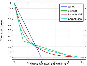
When combined with the crack-band method, the stress versus strain curves in Figure 3-25 are defined in terms of stress versus displacement. The stress versus displacement curves are then converted to unique stress versus strains curves at each material point using the crack-band width hcb, see The Crack Band Method.

In addition to the built-in softening laws, COMSOL Multiphysics allows user-defined definitions of fs(·) and for this purpose provides the variables <phys>.<feat>.<feat>.edmgt and <phys>.<feat>.<feat>.edmgc for the damaged strain in tension and compression, respectively. Alternatively, the user-defined softening behavior can be specified in terms of a stress versus displacement curve fw(·). Equation 3-111 is then replaced by

assuming that the crack-band method is used. If chosen, COMSOL Multiphysics provides the variables <phys>.<feat>.<feat>.wdmgt and <phys>.<feat>.<feat>.wdmgc for the damaged displacement in tension and compression, respectively. For both these options, the a nonlinear equation needs to be solved to find d.