The Semiconductor interface provides the built-in functionality to visualize doping profiles for the selected
Analytic Doping Model or
Geometric Doping Model feature. You can visualize doping profiles by clicking the preview buttons before solving the model. Two buttons named as
 Plot Doping Profile for Selected
 and
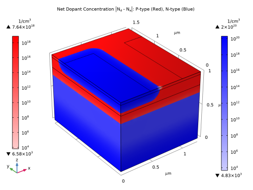
 Plot Net Doping Profile for All
 are available both in the toolbar and the context menu. The doping profile will be shown in a separate plot window named as
 Doping Profile Plot
. Note that p-type and n-type domains are shown in red and blue color, respectively.
The Plot Doping Profile for Selected button visualizes the dopant concentration added by the selected doping feature. The added dopant concentration is defined as
semi.<tag>.Na and
semi.<tag>.Nd for acceptor doping and donor doping, respectively. The
Plot Net Doping Profile for All button visualizes the absolute value of the net dopant concentration defined as
|Nd-Na|.
Note that the plots for doping profiles generated by clicking preview buttons cannot be modified. However, it is also possible to create a customized doping profile. To do this, in the Study toolbar, click
Get Initial Value (

). Then add a plot group and display the corresponding dopant density. The signed doping concentration,
semi.Nd-semi.Na (positive for net donor doping and negative for net acceptor doping), gives the net doping and can be useful for visualizing the effect of different doping steps. If multiple doping features are superimposed, it is possible to visualize the total dopant concentration or to display the contribution from individual doping features.
The semi.Nd-semi.Na expression shows the total net doping due to the sum of all doping features. To see the distribution from a single doping feature the corresponding node tag must be included in the plot variable.
The node tags are shown in curly brackets next to the nodes in the Model Builder. Analytic Doping Model features are tagged as
adm# and
Geometric Doping Model features are tagged as
gdm#, where
# corresponds to the number of the feature. The dopant concentration from each doping feature is available as
semi.<tag>.Na for acceptor doping or
semi.<tag>.Nd for donor doping. For example,
semi.adm1.Nd for a donor distribution from the first
Analytic Doping Model added to the component.