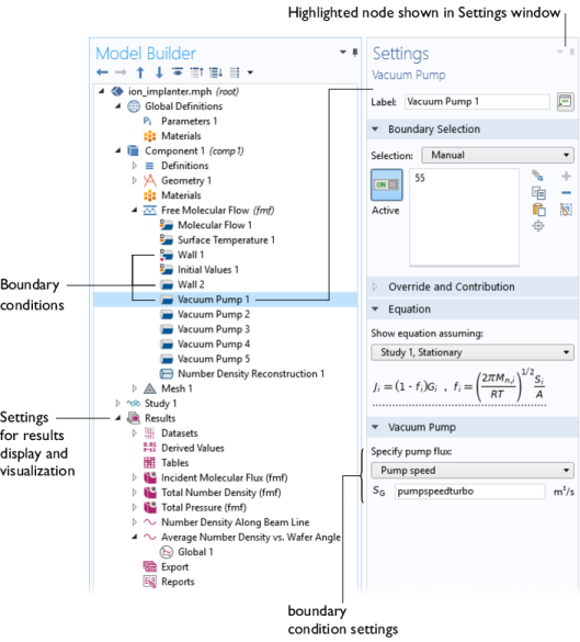
The physics interfaces are used to set up a simulation problem. Each physics interface expresses the relevant physical phenomena in the form of an equation system with appropriate boundary and initial conditions. Each feature added to the interface represents a term or condition in the underlying equation set. These features are usually associated with a geometric entity within the model, such as a domain, boundary, edge (for 3D components), or point. Figure 5 uses the Ion Implanter model (see the section Tutorial Model: Molecular Flow in an Ion Implant Vacuum System) to show the Model Builder and the Settings window for the selected Vacuum Pump 1 node. This node removes a fraction of the incident molecules from the molecular flow in a manner consistent with the pump speed, which is given in liters per second. Note that COMSOL Multiphysics uses SI units by default, but allows quantities to be expressed in other units. Units are entered in square brackets (in this case adding [l/s] after the numeric quantity specifies liters per second). Two different wall boundary conditions are also highlighted in the model tree. Different options are used in these boundary conditions to specify various interactions with the flow. Wall 1 uses the Wall option, which sets the incident molecular flux, G, equal to the emitted molecular flux, J. Wall 2 uses the Outgassing Wall option and correspondingly emits an outgassing molecular flux, J0, in addition to the incident flux, G. J0 can be specified as a flux (SI unit: 1/(m2·s)), a mass flux (SI unit: kg/(m2·s)), a total mass flow (SI unit: kg/s) or as a mass flow in sccm units.

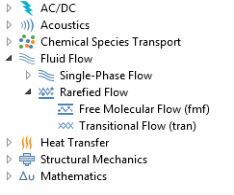
When a new model is started, the appropriate physics interface is selected from the Model Wizard. Figure 6 shows the Molecular Flow Module physics interfaces as displayed in the Model Wizard. Also see Physics Interface Guide by Space Dimension and Preset Study Type. In the following section, a brief overview of each of the Molecular Flow Module physics interfaces is given.

At large Knudsen numbers (Kn > 10), the Molecular Flow interface () can be used. This interface models nonisothermal or isothermal molecular flows using a technique called the angular coefficient method. In this method, the incoming molecular flux at an area element on the surface is computed by summing the outgoing flux arriving from all other visible points. The method is also known as the ‘radiation method’ since previously software for computing surface–to–surface radiation was adapted for this purpose. Note that the Molecular Flow interface is different from the standard radiation method, as it computes accurate pressure and number densities by performing additional integrations. It is also much more convenient, because it is designed specifically for vacuum applications. A limitation of the angular coefficient method is that the boundary conditions on surfaces require the assumption that the molecules are reemitted at directions independent of their angle of incidence. This is often referred to as total accommodation, and is implicitly assumed by the Molecular Flow interface.

COMSOL Multiphysics also offers a Slip Flow interface for modeling nonisothermal or isothermal gas flows in the near continuum regime (0.01 < Kn < 0.1). This physics interface is available in the Microfluidics Module.