Domain Decomposition (Schur)

The node (

) is an attribute node that can be used together with the Iterative and Coarse Solver nodes. Use it to set up a domain-decomposition solver using the Schur complement method. Domain decomposition divides the modeling domain into subdomains where the equations in the subdomains are easier to solve. The total solution is then obtained by iterating between the computed solutions for each subdomain using the currently known solutions from the other subdomains as boundary conditions. The domain decomposition (Schur) solver is a typically more stable but less memory efficient alternative to the domain decomposition (Schwarz) solver.

Default Schur Solver, Domain Solver, and Schur Source Solver nodes are also added. The domain can be any of the direct and iterative solvers, and also a geometric multigrid solver. When you use a multigrid solver as the domain solver for domain decomposition, each domain solves an independent linear problem using a multigrid solver. Each linear problem is created from the underlying multigrid solver’s mesh case hierarchy. The domain problems can then be solved independently. See also The Domain Decomposition Solvers.

Select a : (the default) or . These ordering options determine which corresponding Schwarz algorithm (see Domain Decomposition (Schwarz)) to use for solving the Schur complement system. Schur ordering is not used if absorbing boundary conditions are selected; see The Domain Decomposition Solvers.

For any , enter values or choose an option as needed:

•

. The default is 4. The subdomain partition is created from an element partition on the solver level.

•

. The default is 100,000 DOFs. The solver tries to not create subdomains larger than this and increases the number of subdomains to fulfill the target. The lowest value accepted is 1000.

•

. The default is 1. This option is only relevant in cluster computations. Each subdomain is then handled by the selected number of compute nodes.

•

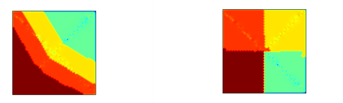
: (the default), , or . The option creates a subdomain distribution by means of the element and vertex lists taken from the mesh. This option typically gives a low number of colors and gives balanced subdomains (equal number of DOFs, small subdomain interfaces, and a smaller overlap if extended). To avoid slim domains, you can also use a preordering algorithm based on a . The following plots show a 2D subdomain configuration without element preordering (left) and with an element reordering based on a space-filling curve (right):

•

Choose an option from the list if required: (default), , or . The option is a computationally expensive option because the subdomain problems are factorized for each iteration and then cleared from memory. If you use the option, the recompute and clear mechanism is activated if there is an out-memory-error during the domain decomposition setup phase. The setup is then repeated with recompute and clear activated. A warning is given in this case.

•

If is selected as the , the check box is selected by default to use a coloring technique that leads to more efficient computations for the multiplicative method because it requires the global residual to be updated after each subdomain. The coloring technique gives each subdomain a color such that subdomains with the same color are disjoint and can be computed in parallel before the residual is updated. Click to clear the check box as needed.

•

In the list, include the geometries (components) in the model that you want to partition using domain decomposition. By default, this list includes all geometries in the model. Use the (

), (

), and (

) buttons to configure the lists of geometries.

•

The check box is selected by default to include extra dimension in the domain decomposition partitioning in models that include extra dimensions. Clear the check box to exclude any extra dimensions from the partitioning.

•

Select the check box to visualize the domains in the domain decomposition using a surface plot, for example. The plot then shows the numbering of the domains instead of the physics solution. A node appears in the solver configuration under the node to inform you that the solution can only be used to visualize domains in the domain decomposition. You will then have to re-solve the model to postprocess the physics in the model.

From the list, choose a boundary condition: , , or .

If you have selected the , then select:

: The code internally creates an for the selected physics. Specify a zero-order coefficient as a scalar value in the field (default: 0.75). You can add a second-order term by selecting the check box and specifying a (default: 0.005). These coefficients correspond to α and β, respectively, in the following equation for an absorbing boundary condition:

The option is only supported for the Helmholtz equation. Select the check box in order to keep the feature in the Physics node.

: Specify the complete weak-form expression in the field. This expression can be applied to any Physics available in the list above. Select the check box to keep the feature in the Physics node.

: the is taken from the Physics node. Only use this option if a weak contribution feature was previously added by selecting the check box together with the or options as described above.

User the settings in the section to set up a hybrid preconditioner where the direct preconditioner is active for some dependent variables. See Hybrid Preconditioners for more information.