|
|
In the COMSOL Multiphysics Reference Manual see the Theory for the Boundary Elements PDE section for more information about the Boundary Element Method.
|
|
|
If both The Electromagnetic Waves, Frequency Domain Interface and The Electromagnetic Waves, Boundary Elements Interface are available, the Electric Field Coupling node is available from the Multiphysics menu in the Physics toolbar or by right-clicking the Multiphysics Couplings node in Model Builder.
|
|
|
The Electromagnetic Waves, Frequency Domain Interface and The Electromagnetic Waves, Boundary Elements Interface can also be coupled by using the same name for the dependent variable for both interfaces. Then Electric Field Coupling is not needed. How to set the name for the dependent variable is described in the Dependent Variables section.
|
|
|
In the COMSOL Multiphysics Reference Manual see the Physics-Controlled Mesh section for more information about how to define the physics-controlled mesh.
|
|
|
For more information about making selections, see Working with Geometric Entities in the COMSOL Multiphysics Reference Manual.
|
|
•
|
Three-component vector (the default) to solve using a full three-component vector for the electric field E.
|
|
•
|
Out-of-plane vector to solve for the electric field vector component perpendicular to the modeling plane, assuming that there is no electric field in the plane.
|
|
•
|
In-plane vector to solve for the electric field vector components in the modeling plane assuming that there is no electric field perpendicular to the plane.
|
|
|
The scattered field formulation supports both metallic PEC scatterers and dielectric scatterers. Notice that a Wave Equation, Electric can be active on multiple domains provided that each material parameter (Relative permittivity, Relative permeability, and Electrical conductivity) has the same constant value in all the selected domains. In brief, there needs to be a Wave Equation, Electric node for each dielectric material.
When multiple Wave Equation, Electric nodes exist, the Infinite void selection needs to correspond to the first Wave Equation, Electric node and cannot coexist with other domain selections.
|
|
|
Optical Yagi–Uda Antenna: Application Library path Wave_Optics_Module/Optical_Scattering/optical_yagi_uda_antenna demonstrates how to use the Scattered field formulation with domain scatterers.
|
|
|
|
|
Evanescent waves are included in the plane wave expansion if the Maximum transverse wave number kt,max is larger that the specified Wave number k. When the Wave vector distribution type is set to Automatic, evanescent waves are included in the expansion if the Allow evanescent waves check box is selected.
|
|
•
|
Select a Beam orientation: Along the x-axis (the default), Along the y-axis, or for 3D components, Along the z-axis.
|
|
•
|
|
•
|
|
•
|
|
•
|
Enter the component expressions for the Transverse background electric field amplitude, Gaussian beam ETbg0 (SI unit: V/m) if the Input quantity is Electric field amplitude. Notice that this is the transverse Gaussian beam amplitude in the focal plane. When the Gaussian beam type is set to Paraxial approximation the background field is always orthogonal (transverse) to Beam orientation. However, when the Gaussian beam type is set to Plane wave expansion, the background field amplitude can also have a component in the propagation direction. Specify here only the field amplitude components that are orthogonal to the propagation direction. COMSOL computes automatically the component in the propagation direction, if needed.
|
|
•
|
If the Input quantity is set to Power, enter the Input power (SI unit: W in 2D axisymmetry and 3D and W/m in 2D) and the component expressions for the Non-normalized transverse electric field amplitude, Gaussian beam ETbg0 (SI unit: V/m).
|
|
•
|
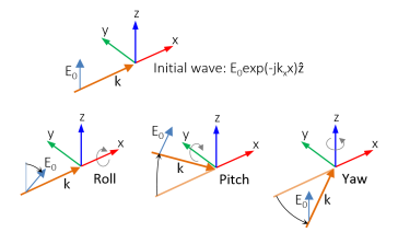
Enter a Wave number k (SI unit: rad/m). The default is ebem.k0 rad/m. The wave number must evaluate to a value that is the same for all the domains the scattered field is applied to. Setting the Wave number k to a positive value, means that the wave is propagating in the positive x-, y-, or z-axis direction, whereas setting the Wave number k to a negative value means that the wave is propagating in the negative x-, y-, or z-axis direction.
|
|
•
|
|
•
|
Enter a Roll angle (SI unit: rad), which is a right-handed rotation with respect to the +x direction. The default is 0 rad, corresponding to polarization along the +z direction.
|
|
•
|
Enter a Pitch angle (SI unit: rad), which is a right-handed rotation with respect to the +y direction. The default is 0 rad, corresponding to the initial direction of propagation pointing in the +x direction.
|
|
•
|
Enter a Yaw angle (SI unit: rad), which is a right-handed rotation with respect to the +z direction.
|
|
•
|
Enter a Wave number k (SI unit: rad/m). The default is ebem.k0 rad/m. The wave number must evaluate to a value that is the same for the domains the scattered field is applied to.
 |
|
|
For more information about the Far Field Approximation settings, see Far-Field Approximation Settings in the COMSOL Multiphysics Reference Manual.
|
|
|
For more information about the Quadrature settings, see Quadrature in the COMSOL Multiphysics Reference Manual.
|