The axial strain εn is calculated by expressing the global strains in tangential derivatives and projecting the global strains on the edge.

where t is the edge tangent vector and εgT is defined as

The constitutive relation for a truss is uniaxial. The axial stress, σn, is computed as

For output, the First Piola-Kirchhoff stress Pn is computed from the Second Piola-Kirchhoff stress using

where s’ is the ratio between current and initial length. The axial force in the element is then computed as

where A0 is the undeformed cross-section area. The engineering (Cauchy) stress is defined by

where A is the deformed area of the element. For a geometrically linear analysis, the change in area is ignored, so that A = A0.

For a geometrically nonlinear analysis, the area change is computed based on an assumption about a linear elastic material with Poisson’s ratio ν. The area change is

This is the only occasion where the Truss interface makes use of the value of ν.

where the summation stands for summation over all points in the geometry. Replacing the integration over the cross section with the cross-sectional area (A) and the volume forces with line forces, the equation becomes

Starting with the large displacement case, let xd1 and xd2 be the deformed position of the two endpoints of the edge

where ui is the displacement, and xi is the coordinate (undeformed position) at endpoint i. The equation for the straight line through the endpoints is

where t is a parameter along the line, and a is the direction vector for the line. a is calculated from the deformed position of the endpoints as

The constraints for the edge are derived by substituting the parameter t from one of the scalar equations in Equation 10-3 into the remaining ones. In 2D the constraint equations become

This constraint is nonlinear, since a depends on the displacement.

where uax is the axial displacement along the edge, and xn is a linear parameter along the edge

Eliminating uax from Equation 10-4 results in the following linear constraint in 2D

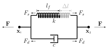
You can use a Spring-Damper Material to connect two points by an elastic spring, a viscous damper, or both. Such springs can be used in any structural mechanics physics interface, by adding a Truss interface. You can then set the degree of freedom names in the two interfaces to the same name, in order to share the same displacement fields.

The current position of the two endpoints, x1 and x2 can be written as

where X1 and X1 are the original positions of the two points, and u1 and u2 are their respective displacements. The initial spring length, l0, is

The current spring length, l, is

In addition to the initial geometrical distance between the two points you can specify an initial spring extension Δl0, so that the free length of the spring is

The spring extension Δl is computed as the difference between the current spring length and the free length,

You can specify that the Spring-Damper Material should be deactivated under certain conditions. It can for example be active only in tension, or break at a certain elongation. In terms of implementation, this means that many expressions are multiplied by an activation indicator, iac. The activation indicator has the value 1 when the component is active, and 0 when deactivated.

The spring force is proportional to the spring constant k:

If k depends on the extension, so that the spring is nonlinear, it should be interpreted as a secant stiffness, that is

To create the expression for the function, use the built-in variable for the spring extension. It has the form <physicsTag>.<SpringNodeTag>.dl, for example truss.spd1.dl.

where c is the viscous damping coefficient. In frequency domain, it is also possible to specify a loss factor η, and the total damping force will then be

In a time-dependent analysis, the energy dissipated in the damper, Wd, is computed using an extra degree of freedom. The following equation is added:

Here, E is Young’s modulus, Imin is the area moment of inertia in the weakest orientation of the cross section, and L is the length of the bar. K is called the effective length factor, and can be used to compensate for non-ideal end conditions. The value 1 corresponds to the Euler 2 buckling case, in which both ends are pinned.

The failure index is computed as the ratio between the compressive axial force N and the critical load:

A failure index exceeding 1 means that the buckling load is exceeded. A set of variables providing different measures of the utilization is listed in Table 10-1.