The Shell and Plate Interfaces

The interface (

), found under the branch (

) when adding a physics interface, is used to model structural shells on boundaries in 3D or 2D axisymmetry. Shells are thin flat or curved structures, having significant bending stiffness. The interface uses shell elements of the MITC type, which can be used for analyzing both thin (Kirchhoff theory) and thick (Mindlin theory) shells.

The interface (

), found under the branch (

) when adding a physics interface, provides the ability to model structural plates in 2D. Plates are thin flat structures with significant bending stiffness, being loaded in a direction out of the plane.

	The Shell interface is for 3D and 2D axisymmetry models. The Plate interface is for 2D models — domains are selected instead of boundaries, and boundaries instead of edges. Otherwise the Settings windows are similar to those for the Shell interface.

The Linear Elastic Material is the default material model. It adds a linear elastic equation for the displacements and has a Settings window to define the elastic material properties. With this material model, the material is assumed to be homogeneous through the thickness of the shell.

When this interface is added, these default nodes are also added to the — , , (a boundary condition where edges are free, with no loads or constraints), and . Then, from the toolbar, add other nodes that implement, for example, boundary conditions. You can also right-click or to select physics features from the context menu.

The is the default physics interface name.

The is used primarily as a scope prefix for variables defined by the physics interface. Refer to such physics interface variables in expressions using the pattern <name>.<variable_name>. In order to distinguish between variables belonging to different physics interfaces, the name string must be unique. Only letters, numbers, and underscores (_) are permitted in the field. The first character must be a letter.

The default (for the first physics interface in the model) is shell or plate.

In the section, a conceptual sketch of the degrees of freedom in the Shell and Plate interfaces appears.

	Select Circumferential mode extension to prescribe a circumferential wave number to be used in eigenfrequency or frequency-domain studies. When selected, enter the Azimuthal mode number m. For more information, see Circumferential Displacement and Out-of-Plane Waves in the Structural Mechanics Theory chapter.

	Eigenfrequency Analysis of a Free Cylinder: Application Library path Structural_Mechanics_Module/Verification_Examples/free_cylinder.

From the list, select (the default) or . Use to treat the dynamic behavior as quasi static (with no mass effects; that is, no second-order time derivatives). Selecting this option gives a more efficient solution for problems where the variation in time is slow when compared to the natural frequencies of the system. The default solver for the time stepping is changed from Generalized alpha to BDF when is selected.

For problems with creep, and sometimes viscoelasticity, the problem can be considered as quasistatic. This is also the case when the time dependence exists only in some other physics, like a transient heat transfer problem causing thermal strains.

	This section is available for the Shell interface only. Also see The MITC Shell Formulation.

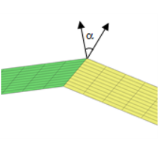
The fold-line limit angle α is the smallest angle between the normals of two boundaries that makes their intersection to be treated as a fold line. The normal to the shell is discontinuous along a fold-line. Enter a value or expression in the α field. The default value is 0.01 radians (approximately 0.6 degrees). The value must be larger than 0, and less than π/2, but angles larger than a few degrees are not usually meaningful.

Since the rotational degrees of freedom have different meaning across a fold line, they are separate degrees of freedom, which a joined by a constraint. This constraint is, as default, implemented as a pointwise constraint. Select to use a weak constraint instead.

Enter a number between -1 and 1 for the Z. The value can be changed from −1 (downside) to +1 (upside). The default is +1. A value of 0 means the midsurface of the shell. This is the default position for stress and strain evaluation during the results analysis. During the results and analysis stage, the coordinates can be changed in the section in the result features.

To display this section, click the button (

) and select in the dialog box. Normally these settings do not need to be changed.

The check box is selected by default, and this interpolation, which is part of the MITC shell formulation, should normally always be active.

	For the Plate interface, the Use 3D formulation check box is used to select whether six or three variables are used in the formulation. For geometrically nonlinear analyses, or when in-plane (membrane) forces are active, six variables must be used. This check box is selected by default.

	As a default, a selective integration scheme is used for the weak contributions used to form the stiffness matrix in 2D axisymmetry. The membrane part of the strain energy is integrated using reduced integration in order to remove locking effects for thin shells. Deselect the Use reduced integration scheme check box to use full integration instead.

In order to maintain the property that the shell normal has unit length, a constraint is applied on the shell normal displacement degrees of freedom in each node. This constraint is, as default, implemented as a pointwise constraint. Select to use a weak constraint instead.

You can chose how to group in the solver nodes the extra ODE variables added by some features.

Select the check box to group in the solver node the variables added by the Rigid Connector feature.

Select the check box to group in the solver node the variables added by the Attachment feature.

The selection made in the section can be overridden by the settings in the section of the Rigid Connector or Attachment features.

This section will only be displayed if a mesh on NASTRAN® format, containing RBE2 elements, has been imported in an node under . The purpose is to automatically create rigid connectors from RBE2 elements in the NASTRAN file.

An RBE2 element represents a rigid connection between a set of mesh nodes. This means that it can, and often does, connect elements from different physics interfaces.

In the drop-down menu in the section title, you can select . The effect is that one rigid connector will be created for each RBE2 element in the imported file. This will happen for all physics interfaces in the list. Supported interfaces are: Solid Mechanics, Shell, Beam, and Multibody Dynamics. If there are RBE2 elements spanning more than one physics interface, they will be automatically connected.

The created rigid connectors will have point, edge, and boundary selections as inferred from the nodes in the RBE2 element and the mesh connectivity. The ‘independent node’ of the RBE2 element is used as center of rotation for the rigid connector.

The section is present in the Solid Mechanics, Shell, and Beam interfaces. In a model that contains several physics interfaces, you should use the automated model setup from only one of them, and make sure that all the involved interfaces are selected in the list.

Select the order of the — or . The degrees of freedom for the displacement of the shell normals will always have the same shape functions as the displacements.

Both interfaces define two dependent variables (fields) — the displacement field u and the field of normal displacements ar. The names can be changed, but the names of fields and dependent variables must in general be unique within a model. If you intentionally use the same name for fields from different physics interfaces, these degrees of freedom are treated as being the same. This can be used when mixing different type of structural mechanics interfaces, where you often want the displacements to be the equal.