Self-Focusing

For low intensities, the refractive index is independent of the intensity of the light in the material. However, when the intensity is large, so large that the electric field of the light field actually start to perturb the electron clouds around the nuclei, the refractive index start to depend on the intensity. Thus, for dielectrics, like glass, the refractive index increases with the intensity.

When a Gaussian beam propagates through a medium with an intensity-dependent refractive index, the index is highest at the center of the beam. Thus, the induced refractive index profile acts as a lens or a waveguide that counteracts the spreading of the beam due to diffraction. The effect that the beam itself induces this positive, focusing, lens in the material is called self-focusing.

Self-focusing manifests itself both in terms of whole-beam focusing, where the beam’s properties are changed by the induced index profile, and by small-scale focusing, where noise across the beam’s cross-sectional intensity distribution is amplified and the beam can break up into several self-focused filaments.

The nonlinear refractive index is written as

where n0 is the constant (linear) part of the refractive index, γ is the nonlinear refractive index coefficient and I is the intensity. The nonlinearity is due to the optical Kerr effect, which is a nonlinear distortion of the electron clouds around the nuclei in the material. For the standard optical glass BK-7, the nonlinear coefficient is 4·10-16 cm2/W. Thus, for an intensity of 2.5 GW/cm2, the induced refractive index change is 10-6. This is a small change, but it has a significant effect on the beam parameters.

Self-focusing is important from a laser engineering perspective, as the modification of the beam must be incorporated in the design. Furthermore, if the threshold for self-focusing is exceeded, the material is damaged. Thus, it is important to know the self-focusing threshold values for the materials used in the design. Self-focusing occurs in dielectrics, like optical glasses and laser rod materials, such as Nd:YAG.

A first estimate of the threshold power for self-focusing is obtain by assuming that the beam has a circular cross-section with a uniform intensity. Within this beam, the refractive index is higher than outside the beam. Thus, the beam itself induces a waveguide structure. You can equal the acceptance angle of the waveguide with the diffraction angle from the circularly confined light. From this equality, you get the critical power to be

(1)

Model Definition

The geometry for the model is simple — just a cylinder.

The incident beam is approximated by a Gaussian beam¹, polarized in the z direction. The electric field is given by

where E0 is the electric field amplitude, w0 is the spot radius at the waist, k is the wave number, defined by k = 2πn0/λ, and z is the unit vector in the z direction. The function w(x) defines the spot size variation as a function of the distance from the beam waist,

(2)

where x0 = πn0w02/λ is the Rayleigh range. The radius of curvature is defined by

and the phase change close to the beam waist, the so-called Gouy shift, is defined by

Results and Discussion

Figure 1 shows the Gaussian beam for a low input intensity. As expected, the beam is symmetric around the beam waist location.

Figure 1: The Gaussian beam for a low peak intensity, I0 = 1 kW/cm2.

Figure 2 shows the beam for a high input intensity, I0 = 14 GW/cm2. The nominal induced refractive index, γI0, is 5.6×10-6. As noted from Figure 3 the actual induced refractive index is much larger than the nominal value. This is of course an effect of the self-focusing of the beam.

Figure 2: The Gaussian beam for a high peak intensity, I0 = 14 GW/cm2.

To demonstrate the effect of self-focusing, Figure 4 shows the calculated spot radius at the boundary between the propagation domain and the PML domain. The spot radius is defined by

(3)

where A is the integration area and I(y,z) is the cross-sectional intensity distribution of the beam. For low peak intensities, the calculated spot radius, using Equation 3, give similar results as the Gaussian beam expression in Equation 2. However, with increasing intensities, the beam start to deviate from a Gaussian beam and the spot radius is reduced linearly with intensity.

Figure 3: The induced refractive index change, γI, for a high peak intensity, I0 = 14 GW/cm2.

Figure 4: The spot radius at the end of the propagation domain versus the peak intensity.

The final intensity used in the parametric sweep is 14 GW/cm2. This corresponds to a power that is 23% of the critical power, provided in Equation 1. As discussed in Ref. 1, it is expected that the critical power for a Gaussian beam is reduced by a factor of approximately 4/(1.22π)2 = 0.27. Thus, the power corresponding to the last peak intensity in the sweep is approximately a factor 0.23/0.27 = 0.85 from the critical power for self-focusing for a Gaussian beam, where the induced refractive index profile completely balances the diffractive spreading of the beam.

To compute the field for even higher intensities, a much finer mesh would be needed, as the beam can break up into filaments. For a nonlinear problem like this, it is important to verify the results by, for instance, repeating the simulation with a finer mesh.

Reference

1. W. Koechner, Solid-State Laser Engineering, Springer, chap. 4.6, 2010.

Wave_Optics_Module/Nonlinear_Optics/self_focusing

Modeling Instructions

From the menu, choose .

New

In the window, click

Model Wizard

In the window, click

In the tree, select .

Click .

Click

In the tree, select .

Click

Global Definitions

Start by adding some global model parameters.

Parameters 1

In the window, under click .

In the window for , locate the section.

In the table, enter the following settings:


Name	Expression	Value	Description
lda0	1.064[um]	1.064E-6 m	Wavelength
w0	100*lda0	1.064E-4 m	Nominal spot radius
n0	1.52	1.52	Refractive index of BK-7 glass
x0	pin0w0^2/lda0	0.050808 m	Rayleigh range
k	2pin0/lda0	8.976E6 1/m	Propagation constant
I0	2.5[GW/cm^2]	2.5E13 W/m²	Nominal peak intensity
E0	sqrt(2I0/n0sqrt(mu0_const/epsilon0_const))	1.1132E8 V/m	Nominal peak electric field
length	4*x0	0.20323 m	Length of computation domain
radius	2.5w0sqrt(1+(length/(2*x0))^2)	5.9479E-4 m	Radius of computation domain
gamma	4e-16[cm^2/W]	4E-20 s³/kg	Nonlinear refractive index coefficient
delta_n	gamma*I0	1E-6	Nominal refractive index change
P_cr	(1.22pi)^2lda0^2/(8pin0*gamma)	1.0883E7 W	Critical power

Geometry 1

Cylinder 1 (cyl1)

In the toolbar, click

In the window for , locate the section.

In the text field, type radius.

In the text field, type length.

Locate the section. In the text field, type -length/2.

Locate the section. From the list, choose .

Block 1 (blk1)

Since the planes y = 0 and z = 0 should be symmetry planes for the beam, we only need to model one forth of the beam. Thus, add a block that intersect one quadrant of the cylinder.

In the toolbar, click

In the window for , locate the section.

In the text field, type length.

In the text field, type radius.

Locate the section. In the text field, type -length/2.

In the text field, type -radius.

Intersection 1 (int1)

In the toolbar, click

and choose .

Click in the window and then press Ctrl+A to select both objects.

In the toolbar, click

Global Definitions

Since the geometry is so long and thin, modify the view settings to not preserve the aspect ratio.

Definitions

In the window, expand the node.

Camera

In the window, expand the node, then click .

In the window for , locate the section.

From the list, choose .

Select the check box.

Click

Click the

button in the toolbar.

Materials

Now add the BK-7 glass used in the model.

BK-7 glass

In the window, under right-click and choose .

In the window for , type BK-7 glass in the text field.

Locate the section. In the table, enter the following settings:


Property	Variable	Value	Unit	Property group
Refractive index, real part	n_iso ; nii = n_iso, nij = 0	n0+gamma*ewbe.Poavx	1	Refractive index

The variable ewbe.Poavx represents the intensity in the propagation direction.

Definitions

Setup a boundary integration operator, for calculation of the output power and the output spot radius.

Integration 1 (intop1)

In the toolbar, click

and choose .

In the window for , type intop_output_boundary in the text field.

Locate the section. From the list, choose .

Select Boundary 5 only.

Variables 1

Add the expressions for the output power and the output spot radius.

In the toolbar, click

In the window for , locate the section.

In the table, enter the following settings:


Name	Expression	Unit	Description
P	intop_output_boundary(ewbe.nPoav)	W	Output power
w_t	sqrt(2intop_output_boundary(ewbe.nPoav(y^2+z^2))/P)	m	Spot radius on output boundary

Electromagnetic Waves, Beam Envelopes (ewbe)

Set the interface to use unidirectional propagation and define the wave vector component in the x direction.

In the window, under click .

In the window for , locate the section.

From the list, choose .

Specify the k1 vector as


k	x
0	y
0	z

Use a matched boundary condition to launch an incident Gaussian beam polarized in the z direction.

Matched Boundary Condition 1

In the toolbar, click

and choose .

Select Boundary 1 only.

In the window for , locate the section.

From the list, choose .

In the w0 text field, type w0.

In the p0 text field, type length/2.

From the list, choose .

In the P text field, type pi*w0^2/2*I0.

Specify the Eg0 vector as


0	x
0	y
1[V/m]	z

Add a reference point that together with the propagation direction defines the optical axis.

Reference Point 1

In the toolbar, click

and choose .

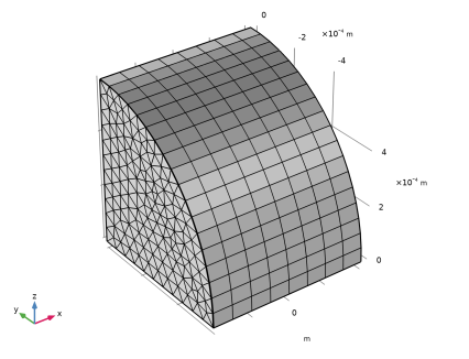
Select Point 2 only, that is the point on the optical axis (where y = 0 and z = 0). The focal point is located the distance p0 from this reference point in the propagation direction, defined by ewbe.k1.

Matched Boundary Condition 2

In the toolbar, click

and choose .

Select Boundary 5 only.

Symmetry Plane 1

Add a perfect magnetic conductor symmetry plane on the plane y = 0 and a perfect electric conductor symmetry plane on the plane z = 0.

In the toolbar, click

and choose .

Select Boundary 4 only.

Symmetry Plane 2

In the toolbar, click

and choose .

Select Boundary 2 only.

In the window for , locate the section.

From the list, choose .

Mesh 1

The physics-controlled meshing cannot handle the nonlinear refractive index defined for the BK-7 material. Thus, create a custom mesh. First create a triangular mesh on the input boundary and then a swept mesh for the domain.

Free Triangular 1

In the toolbar, click

and choose .

Size

Set the main settings to represent the discretization along the propagation direction. Since the beam is expected to behave as a slightly distorted Gaussian beam, it is sufficient to set the maximum mesh element size to half the Rayleigh range.

In the window, click .

In the window for , locate the section.

Click the button.

Locate the section. In the text field, type x0/2.

Free Triangular 1

In the window, click .

Select Boundary 1 only.

Size 1

Right-click and choose .

The triangular mesh should resolve the beam cross-sectional distribution.

In the window for , locate the section.

Click the button.

Locate the section.

Select the check box. In the associated text field, type w0/2.

Select the check box. In the associated text field, type w0/4.

Create a swept mesh in the propagation direction.

Swept 1

In the toolbar, click

In the window, right-click and choose .

Study 1

Do not generate the default plots.

In the window, click .

In the window for , locate the section.

Clear the check box.

Step 1: Wavelength Domain

In the window, under click .

In the window for , locate the section.

In the text field, type lda0.

Parametric Sweep

Set up a parametric sweep of the nominal peak intensity, from 1 kW/cm2 (corresponding to linear propagation) to 14 GW/cm2 that will show a significant self-focusing effect.

In the toolbar, click

In the window for , locate the section.

Click

In the table, enter the following settings:


Parameter name	Parameter value list	Parameter unit
I0 (Nominal peak intensity)	1e7, 2e13, 5e13, 8e13, 11e13, 14e13	W/m^2

Click to expand the section. From the list, choose , to turn off the parametric solver that otherwise would perform calculations also for intermediate intensities.

Solution 1 (sol1)

Since this is a nonlinear problem, it is better to split the complex electric field variable into its real and imaginary parts. This will produce a more accurate Jacobian for the problem, leading to a faster convergence.

In the toolbar, click