PDF

Orbital Angular Momentum Beam
Introduction
It is well known that light has energy. The photon has an energy of hν, where h is the Planck constant and ν is the frequency. It is also known that the photon, even though it is a massless particle, possesses a linear momentum. That is, it exerts a force in its propagation direction. This knowledge has led to ideas of spacecraft propulsion based on the radiation pressure from sunlight hitting large mirrors — so called solar sails.
Light also possesses angular momentum in two different forms — spin angular momentum and orbital angular momentum (OAM). Spin angular momentum is associated with the light field polarization. For circular polarization, the electric and magnetic field vectors rotate as the wave propagates. Orbital angular momentum, on the other hand, is related to the wave’s spatial field distribution and in particular the spiraling (helical) phase distribution. The discovery that light also possesses OAM is quite recent. The first paper was published as late as 1992 (see Ref. 1). An introduction to the field of OAM waves and its development since 1992 is found in Ref. 2.
This phase distribution produces a Gaussian donut beam (c.f. Figure 1).
Figure 1: The electric field norm, showing the ring structure of the beam.
As shown in Figure 2, the phase rotates around the optical axis as the beam propagates.
Figure 2: Phase distribution at five different locations along the direction of propagation. As shown, the phase twists as the beam propagates.
The resulting beam, also called a vortex beam or a helical beam, has a spiraling phase distribution as shown in Figure 3 below.
Figure 3: The spiraling phase variation of the vortex (OAM) beam.
One way of creating a beam with OAM is to send a Gaussian beam through a phase plate with a spiraling thickness. Thereby, the transmitted beam will get a spiraling phase front, resulting in a vortex beam.
Since vortex beams with different twists do not interfere with each other, the use of these waves for communication has become a very active research topic. For more information, see Ref. 3.
Model Definition
This model simulates a Laguerre–Gaussian beam with the Electromagnetic Waves, Beam Envelopes interface, using the unidirectional wave formulation. The input beam is a focused Gaussian beam with a spiral phase distribution.
For a wave propagating in the x-direction and with a transverse radial coordinate r, the Laguerre–Gauss field distribution is given by
(1)
where the spot radius varies as the wave propagates as
(2)
and the wave front curvature evolves as
.
Here x0 = πn0w02/λ is the Rayleigh range, k is the wave number, is a generalized Laguerre polynomial with radial mode number m and angular mode number n. The phase function is now
(3).
This model simulates a beam with radial mode number 0 and angular mode number 1. This beam will have one radial node, located on the optical axis. The generalized Laguerre polynomial for this mode is
(4).
Comparing Equation 1with the field distribution for the lowest order Gaussian beam (for example see the Application Library model Self-Focusing), makes it possible to identify that
(5).
Thus, in the model, the expression
(6)
will be used as the Gaussian beam input amplitude.
References
1. L. Allen and others, “Orbital angular momentum of light and the transformation of Laguerre-Gaussian laser modes,” Physical Review A, vol.–45, no.–11, pp.–8185–8189, 1992.
2. S.M. Barnett, M. Babiker, and M.J. Padgett, “Optical orbital angular momentum,” Philosophical Transactions of the Royal Society A, vol. 375, https://doi.org/10.1098/rsta.2015.0444, 2017.
3. A.E. Willner, “Twisted light could dramatically boost data rates,” IEEE Spectrum, vol. 53, no. 8, pp. 34–39, 2016.
Application Library path: Wave_Optics_Module/Beam_Propagation/orbital_angular_momentum
Modeling Instructions
From the File menu, choose New.
New
In the New window, click  Model Wizard.
Model Wizard
1
In the Model Wizard window, click  3D.
2
In the Select Physics tree, select Optics>Wave Optics>Electromagnetic Waves, Beam Envelopes (ewbe).
3
Click Add.
4
Click  Study.
5
In the Select Study tree, select Preset Studies for Selected Physics Interfaces>Wavelength Domain.
6
Global Definitions
Parameters 1
1
In the Model Builder window, under Global Definitions click Parameters 1.
2
In the Settings window for Parameters, locate the Parameters section.
3
Geometry 1
Cylinder 1 (cyl1)
1
In the Geometry toolbar, click  Cylinder.
2
In the Settings window for Cylinder, locate the Size and Shape section.
3
In the Radius text field, type 3*w0.
4
In the Height text field, type 3*lda0.
5
Locate the Axis section. From the Axis type list, choose x-axis.
6
Click  Build All Objects.
Definitions
This view is very compressed in the propagation direction. The following instructions change the Camera’s View scale to make the domain expand in the x direction.
In the Model Builder window, expand the Component 1 (comp1)>Definitions node.
Camera
1
In the Model Builder window, expand the Component 1 (comp1)>Definitions>View 1 node, then click Camera.
2
In the Settings window for Camera, locate the Camera section.
3
From the View scale list, choose Manual.
4
In the x scale text field, type 50.
5
Click  Update.
6
Click the  Zoom Extents button in the Graphics toolbar.
Materials
Air
1
In the Model Builder window, under Component 1 (comp1) right-click Materials and choose Blank Material.
2
In the Settings window for Material, type Air in the Label text field.
3
Locate the Material Contents section. In the table, enter the following settings:
Definitions
Now, add a function and some variables that will be used for defining the input beam.
Spot Radius
1
In the Home toolbar, click  Functions and choose Local>Analytic.
2
In the Settings window for Analytic, type Spot Radius in the Label text field.
3
In the Function name text field, type w.
4
Locate the Definition section. In the Expression text field, type w0*sqrt(1+(x/zR)^2).
5
Locate the Units section. In the table, enter the following settings:
6
In the Function text field, type m.
Beam Variables
1
In the Model Builder window, right-click Definitions and choose Variables.
2
In the Settings window for Variables, type Beam Variables in the Label text field.
3
Locate the Variables section. In the table, enter the following settings:
Plot Variables
The following instructions add two variables that later will be used for visualizing the field’s spiraling phase.
1
Right-click Definitions and choose Variables.
2
In the Settings window for Variables, type Plot Variables in the Label text field.
3
Locate the Variables section. In the table, enter the following settings:
Electromagnetic Waves, Beam Envelopes (ewbe)
Set up the physics for unidirectional propagation. Also use the curl type 2 shape function. This makes the problem solve with slightly more degrees of freedom, but the phase plot becomes smoother.
1
In the Model Builder window, under Component 1 (comp1) click Electromagnetic Waves, Beam Envelopes (ewbe).
2
In the Settings window for Electromagnetic Waves, Beam Envelopes, locate the Wave Vectors section.
3
From the Number of directions list, choose Unidirectional.
4
Click to expand the Discretization section. From the Electric field envelopes list, choose Quadratic type 2.
A Matched boundary condition launches a Gaussian beam, defined by the amplitude variable that was previously defined.
Matched Boundary Condition 1
1
In the Physics toolbar, click  Boundaries and choose Matched Boundary Condition.
2
3
In the Settings window for Matched Boundary Condition, locate the Matched Boundary Condition section.
4
From the Incident field list, choose Gaussian beam.
5
In the w0 text field, type w0.
6
Specify the Eg0 vector as
Matched Boundary Condition 2
1
In the Physics toolbar, click  Boundaries and choose Matched Boundary Condition.
2
Mesh 1
1
In the Model Builder window, under Component 1 (comp1) right-click Mesh 1 and choose Build All.
Notice that the curl type 2 shape function does not work with a structured mesh. Thus, the automatically generated swept mesh has automatically been converted to a tetrahedral (unstructured) mesh.
Study 1
Step 1: Wavelength Domain
1
In the Model Builder window, under Study 1 click Step 1: Wavelength Domain.
2
In the Settings window for Wavelength Domain, locate the Study Settings section.
3
In the Wavelengths text field, type lda0.
4
In the Home toolbar, click  Compute.
Results
Electric Field (ewbe)
The plot shows that the beam has a ring structure, with no field on the propagation axis.
Multislice 2
To visualize the spiraling phase distribution, we add a Multislice plot.
1
In the Electric Field (ewbe) toolbar, click  More Plots and choose Multislice.
2
In the Settings window for Multislice, locate the Expression section.
3
In the Expression text field, type argEy.
4
Locate the Multiplane Data section. Find the X-planes subsection. In the Planes text field, type 5.
5
Find the Y-planes subsection. In the Planes text field, type 0.
6
Find the Z-planes subsection. In the Planes text field, type 0.
7
In the Electric Field (ewbe) toolbar, click  Plot.
Inspecting the phase plot, it is clear that the phase becomes noisier in the parts of the beam where the intensity is low. A filter is added to remove the outermost parts of the beam, where the intensity is really low.
Filter 1
1
Right-click Multislice 2 and choose Filter.
2
In the Settings window for Filter, locate the Element Selection section.
3
In the Logical expression for inclusion text field, type rho<2.5*w0.
Electric Field
1
In the Model Builder window, under Results>Electric Field (ewbe) click Electric Field.
2
In the Settings window for Multislice, locate the Multiplane Data section.
3
Find the X-planes subsection. In the Planes text field, type 0.
4
In the Electric Field (ewbe) toolbar, click  Plot.
This phase plot looks clearer.
5
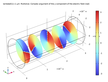
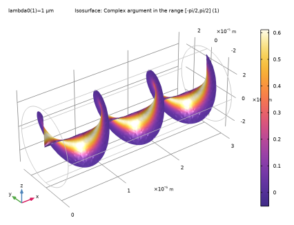
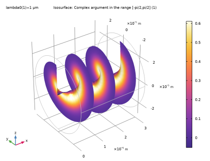
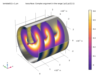
Right-click Results>Electric Field (ewbe)>Electric Field and choose Disable, to only display the phase plot.
Electric Field (ewbe)
1
In the Model Builder window, click Electric Field (ewbe).
2
In the Electric Field (ewbe) toolbar, click  Plot.
3
Click the  Zoom Extents button in the Graphics toolbar.
Phase Plot
The following instructions generate a plot of the spiraling phase.
1
In the Home toolbar, click  Add Plot Group and choose 3D Plot Group.
2
In the Settings window for 3D Plot Group, type Phase Plot in the Label text field.
3
Locate the Plot Settings section. From the Color list, choose Gray.
Isosurface 1
1
Right-click Phase Plot and choose Isosurface.
2
In the Settings window for Isosurface, locate the Expression section.
3
In the Expression text field, type argWindow, which is the phase variable we previously defined.
4
Locate the Levels section. In the Total levels text field, type 1, to display just one isosurface.
5
Click to expand the Quality section. From the Resolution list, choose Finer.
6
Clear the Use derivatives check box, to give a smoother plot.
Filter 1
Finally, add the same filter as in the previous plot, but additionally include a term filtering out only the parts of the beam where |arg(Ey)| is less than π/2. This produces a nice looking "corkscrew" phase distribution.
1
Right-click Isosurface 1 and choose Filter.
2
In the Settings window for Filter, locate the Element Selection section.
3
In the Logical expression for inclusion text field, type rho<2.5*w0&&abs(arg(ewbe.Ey))<pi/2.
Color Expression 1
1
In the Model Builder window, right-click Isosurface 1 and choose Color Expression.
2
In the Settings window for Color Expression, locate the Expression section.
3
In the Expression text field, type ewbe.Ey.
4
Locate the Coloring and Style section. Click  Change Color Table.
5
In the Color Table dialog box, select Thermal>HeatCameraLight in the tree.
6
7
In the Phase Plot toolbar, click  Plot.
This plot looks too expanded in the x direction. This is handled by adding a new view for this plot group.
First make sure that the Views node is available under the Results node.
8
Click the  Show More Options button in the Model Builder toolbar.
9
In the Show More Options dialog box, select Results>Views in the tree.
10
11
View 3D 2
In the Model Builder window, under Results right-click Views and choose View 3D.
Camera
1
In the Model Builder window, expand the View 3D 2 node, then click Camera.
2
In the Settings window for Camera, locate the Camera section.
3
From the View scale list, choose Automatic.
4
Click  Update.
Phase Plot
1
In the Model Builder window, under Results click Phase Plot.
2
In the Settings window for 3D Plot Group, locate the Plot Settings section.
3
From the View list, choose View 3D 2.
4
In the Phase Plot toolbar, click  Plot.
5
Click the  Zoom Extents button in the Graphics toolbar.
The plot has now better proportions. The next section improves it further by showing the y component of the electric field on the cylinder internal surface.
Surface 1
1
Right-click Phase Plot and choose Surface.
2
In the Settings window for Surface, locate the Expression section.
3
In the Expression text field, type ewbe.Ey.
4
Click to expand the Title section. From the Title type list, choose None.
5
Locate the Coloring and Style section. Click  Change Color Table.
6
In the Color Table dialog box, select Linear>Cividis in the tree.
7
8
In the Settings window for Surface, locate the Coloring and Style section.
9
Clear the Color legend check box.
Selection 1
1
Right-click Surface 1 and choose Selection.
2
In the Settings window for Selection, locate the Selection section.
3
Click  Paste Selection.
4
In the Paste Selection dialog box, type 2 4 5 in the Selection text field.
5
Surface 2
In the Model Builder window, under Results>Phase Plot right-click Surface 1 and choose Duplicate.
Selection 1
1
In the Model Builder window, expand the Surface 2 node, then click Selection 1.
2
In the Settings window for Selection, locate the Selection section.
3
Click to select the  Activate Selection toggle button.
4
Click  Clear Selection.
5
Click  Paste Selection.
6
In the Paste Selection dialog box, type 6 in the Selection text field.
7
8
In the Phase Plot toolbar, click  Plot.
Animation 1
The instructions below show how to create an animation of the phase plot.
1
In the Phase Plot toolbar, click  Animation and choose Player.
2
In the Settings window for Animation, locate the Animation Editing section.
3
From the Sequence type list, choose Dynamic data extension.
4
Locate the Playing section. From the Repeat list, choose Forever.
Clicking the Play button in the toolbar for the Graphics window starts the animation. Click the adjacent Stop button to end the animation.