PDF

Leaky Modes in a Microstructured Optical Fiber
Introduction
In a regular optical fiber, light is confined to the core region of the fiber through total internal reflection. That is, the refractive index is higher in the core than in the surrounding cladding. Then if the wave hits the core-cladding interface with an angle from the interface normal that is larger than a certain critical angle, the wave will be perfectly reflected. Thus, ideally, this type of dielectric waveguide is lossless.
By the end of the seventies, it was realized that light could also be guided without relying on total internal reflection. If the core of the fiber was surrounded by concentric layers of materials with alternating high and low refractive indices, the modes can propagate along the fiber without losses, even though the core refractive index is lower than the refractive index of the exterior cladding. This type of fiber is called a Bragg fiber.
Also if you create a regular lattice of air holes in a silica fiber, a similar type of guiding as for the Bragg fiber can be created. This time, though, the guiding occurs through the photonic band gap effect. Consequently, these fibers are called photonic band gap fibers (PBGFs) or photonic crystal fibers (PCFs).
An advantage with these new kinds of fibers is that you can design them to make the guided mode overlap mainly with the air regions. This can potentially reduce the loss in the fiber and it makes the fibers less susceptible to optically nonlinear effects.
In reality, though, the band gap structures and the layer structures cannot be made infinitely large. Thus, there is always some loss associated with the modes in these microstructured optical fibers (MOFs). Thus, when designing these types of fibers, it is of great importance to be able to calculate the loss associated with a certain fiber design.
Model Definition
This model will demonstrate how to use COMSOL for making a mode analysis of a lossy microstructured optical fiber. The geometry is shown in Figure 1.
Figure 1: A microstructured optical fiber. The whole structure consists of silica, except for the small holes that consist of air. The outermost layer is used for the perfectly matched layer (PML), used in the first part of the simulation.
The fiber design implemented in this model has been used in several scientific papers for evaluating different computational methods. See for instance Ref. 1.
Results and Discussion
Figure 2 shows one of the two degenerate HE11-like modes. As this is a mixed mode, both the electric and magnetic field have longitudinal field components, although their magnitude is much smaller than the tangential field components.
Figure 2: This graph shows the norm of the tangential and longitudinal electric and magnetic fields for one of the two degenerate HE11-like modes. To make the longitudinal components visible, they are scaled by a factor of ten relative the tangential field components. The white arrows indicate the tangential electric and magnetic field directions.
This type of fiber is a high-index core fiber, where the core of the fiber has a higher refractive index than the surrounding air-hole ring. Thus, the guiding here could be said to be due to that the local effective index is higher in the core than in the surrounding air-hole ring.
You could also calculate the in-plane wavelength
(1),
where λ is the vacuum wavelength, n is the refractive index of silica, and ni is the effective index of mode i. For the modes with an effective index close to the silica refractive index, the in-plane wavelength will be much larger than the separation between the air holes. Thus, less radiation can leak through the air-hole ring for those modes. When the effective index for the modes decreases, the in-plane wavelength gets smaller and more radiation can leak between the air holes.
Figure 3 shows the TE01-like mode. A pure TE01 mode for a cylindrically symmetric waveguide, has rotational invariance. This TE01-like mode has almost rotational invariance, with the electric field mainly polarized in the  direction whereas the magnetic field has both a radial and longitudinal component.
Figure 3: The TE01-like mode.
Another mode example is the TM01-like mode, shown in Figure 4. Again, the field has almost rotational invariance. However, this time the electric field has both radial and longitudinal components, whereas the magnetic field has mainly a -component.
Figure 4: The TM01-like mode.
Table 1 shows the effective indices for the ten modes found in the mode analysis studies. The first column indicates the mode’s type. The second column, marked with PML, shows the result for the study performed with a PML to truncate the computation domain. The third column, shows the result for the study using a Scattering boundary condition to truncate the computation domain.
As seen in the table, the real parts agree for the first 5–6 decimals, whereas for the much smaller imaginary parts only the orders of magnitude agree. Also when comparing to values reported in Ref. 1, the same kind of agreement is found.
Notes About the COMSOL Implementation
In the first part of the of this simulation, PMLs are used to truncate the simulation domain. To efficiently absorb the wave in the PML, the wavelength corresponding to the wave vector component in the radial direction should be provided. This wavelength is stated in Equation 1 and implemented by the parameter wlr, where an estimation of the largest effective index is used.
In the second part of this modeling task, the Scattering boundary condition is used for truncating the simulation domain. Normally, when the Scattering boundary condition is used, it is assumed that the scattered wave reaching the boundary propagates with a wave vector close to the normal direction to the boundary. However, when we do a mode analysis, we know that the mode will also propagate in the out-of-plane direction, which is tangential to the boundary where the Scattering boundary condition is applied. Thus, the wave vector component in the normal direction to the boundary is
,
where k is the material wave number and β is the propagation constant for the mode. To make sure that this expression is used, enable the Subtract propagation constant from material wave number check box in the Mode Analysis section in the Settings for the Scattering Boundary Condition feature.
Reference
1. H.P. Uranus and H.J.W.M. Hoekstra, “Modelling of microstructured waveguides using a finite-element-based vectorial mode solver with transparent boundary conditions,” Optics Express, vol. 12, no. 12, pp. 2795–2809, 2004.
Application Library path: Wave_Optics_Module/Verification_Examples/microstructured_optical_fiber
Modeling Instructions
From the File menu, choose New.
New
In the New window, click  Model Wizard.
Model Wizard
1
In the Model Wizard window, click  2D.
2
In the Select Physics tree, select Optics>Wave Optics>Electromagnetic Waves, Frequency Domain (ewfd).
3
Click Add.
4
Click  Study.
5
In the Select Study tree, select Preset Studies for Selected Physics Interfaces>Mode Analysis.
6
Global Definitions
Parameters 1
1
In the Model Builder window, under Global Definitions click Parameters 1.
2
In the Settings window for Parameters, locate the Parameters section.
3
Click  Load from File.
4
The parameter wlr, the in-plane wavelength, will be used in the definition of the perfectly matched layer (PML).
Geometry 1
Start building the geometry. Add a circle for the computation domain and then a smaller circle that represents the air holes. The air-hole circle is rotated in steps of 60 degrees. In total, six air holes will be added.
Circle 1 (c1)
1
In the Geometry toolbar, click  Circle.
2
In the Settings window for Circle, locate the Size and Shape section.
3
In the Radius text field, type rb+wlr.
4
Click to expand the Layers section. In the table, enter the following settings:
Circle 2 (c2)
1
In the Geometry toolbar, click  Circle.
2
In the Settings window for Circle, locate the Size and Shape section.
3
In the Radius text field, type d/2.
4
Locate the Position section. In the y text field, type -Delta.
Now, give the selection a name that can be referred to later.
5
Locate the Selections of Resulting Entities section. Find the Cumulative selection subsection. Click New.
6
In the New Cumulative Selection dialog box, type Air Holes in the Name text field.
7
Rotate 1 (rot1)
1
In the Geometry toolbar, click  Transforms and choose Rotate.
2
3
In the Settings window for Rotate, locate the Rotation section.
4
In the Angle text field, type range(0,60,300).
5
Locate the Selections of Resulting Entities section. Find the Cumulative selection subsection. From the Contribute to list, choose Air Holes.
6
Click  Build All Objects.
Add a selection for the air hole boundaries. This selection will be used later, when setting up the plots.
Definitions
Air Hole Boundaries
1
In the Definitions toolbar, click  Adjacent.
2
In the Settings window for Adjacent, type Air Hole Boundaries in the Label text field.
3
Locate the Input Entities section. Under Input selections, click  Add.
4
In the Add dialog box, select Air Holes in the Input selections list.
5
Materials
Now, add the materials.
Silica
1
In the Model Builder window, under Component 1 (comp1) right-click Materials and choose Blank Material.
2
In the Settings window for Material, type Silica in the Label text field.
3
Locate the Material Contents section. In the table, enter the following settings:
Air
1
Right-click Materials and choose Blank Material.
2
In the Settings window for Material, type Air in the Label text field.
3
Locate the Geometric Entity Selection section. From the Selection list, choose Air Holes.
4
Locate the Material Contents section. In the table, enter the following settings:
Definitions
In the first part of the model, a perfectly matched layer (PML) will be used for truncating the computation domain.
Perfectly Matched Layer 1 (pml1)
1
In the Definitions toolbar, click  Perfectly Matched Layer.
2
3
In the Settings window for Perfectly Matched Layer, locate the Geometry section.
4
From the Type list, choose Cylindrical.
5
Locate the Scaling section. From the Typical wavelength from list, choose User defined.
6
In the Typical wavelength text field, type wlr. This parameter approximates the in-plane wavelength.
Study 1
Step 1: Mode Analysis
1
In the Model Builder window, under Study 1 click Step 1: Mode Analysis.
2
In the Settings window for Mode Analysis, locate the Study Settings section.
3
In the Mode analysis frequency text field, type c_const/wl.
4
From the Mode search method list, choose Region, as we will search for the complex effective indices in a rectangular region defined by the following parameters.
5
In the Approximate number of modes text field, type 10.
6
Find the Search region subsection. In the Smallest real part text field, type neffMin.
7
In the Largest real part text field, type neffMax.
8
In the Smallest imaginary part text field, type -3e-5.
Mesh 1
1
In the Model Builder window, under Component 1 (comp1) click Mesh 1.
2
In the Settings window for Mesh, locate the Physics-Controlled Mesh section.
3
From the Element size list, choose Extremely fine.
4
Click  Build All.
The mesh plot shows that the PML domains have been meshed with a mapped mesh.
Study 1
Step 1: Mode Analysis
In the Home toolbar, click  Compute.
Results
Electric Field (ewfd)
1
In the Settings window for 2D Plot Group, locate the Color Legend section.
2
Clear the Show legends check box, as the absolute amplitude of the mode field is not important.
3
In the Electric Field (ewfd) toolbar, click  Plot.
4
Click the  Show Grid button in the Graphics toolbar, to remove some more information that is not necessary in the plot.
5
Click the  Zoom Extents button in the Graphics toolbar.
As seen, the mode field is localized to the central high-index region, with only a very small part of the field penetrating in between the holes.
The effective index is shown in the plot title. As seen, it is a complex number, where the imaginary part represents attenuation of the wave as it propagates along the fiber due to radiation leaking through the air-hole ring. let us evaluate the effective indices for the different modes.
Global Evaluation 1
1
In the Results toolbar, click  Global Evaluation.
2
In the Settings window for Global Evaluation, click Replace Expression in the upper-right corner of the Expressions section. From the menu, choose Component 1 (comp1)>Electromagnetic Waves, Frequency Domain>Global>ewfd.neff - Effective mode index.
3
Click  Evaluate.
Table
1
Go to the Table window.
2
Click Full Precision in the window toolbar.
The imaginary part of the effective index is larger for the modes with a lower real part of the effective index. Those modes have a smaller in-plane wavelength and are, thus, more loosely bound to the central high-index region.
The effective indices in the table should be very close to the values in the second column of Table 1.
Electromagnetic Waves, Frequency Domain (ewfd)
Now, replace the PML with a Scattering boundary condition (SBC).
1
In the Model Builder window, under Component 1 (comp1) click Electromagnetic Waves, Frequency Domain (ewfd).
2
Scattering Boundary Condition 1
1
In the Physics toolbar, click  Boundaries and choose Scattering Boundary Condition.
2
In the Settings window for Scattering Boundary Condition, locate the Boundary Selection section.
3
From the Selection list, choose All boundaries.
4
Locate the Scattering Boundary Condition section. From the Scattered wave type list, choose Cylindrical wave.
5
Click to expand the Mode Analysis section. Select the Subtract propagation constant from material wave number check box, to subtract the mode propagation constant from the material wave number when calculating the wave vector component in the radial (normal) direction.
6
In the Home toolbar, click  Compute.
Results
Global Evaluation 1
1
In the Model Builder window, under Results>Derived Values click Global Evaluation 1.
2
In the Settings window for Global Evaluation, click  Evaluate.
The effective indices in the table should be very close to the values in the third column of Table 1.
Table
1
Go to the Table window.
Comparing the effective indices from the PML and the SBC simulations, it is clear that the real parts agree up to 4–5 decimals, whereas the imaginary parts (that are much smaller in magnitude) only agree by the order of magnitude.
Results
Now, add some additional plots, to make it possible to distinguish the different mode types.
Surface 1
1
In the Model Builder window, expand the Results>Electric Field (ewfd) node, then click Surface 1.
2
In the Settings window for Surface, locate the Expression section.
3
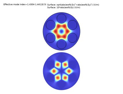
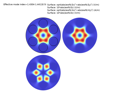
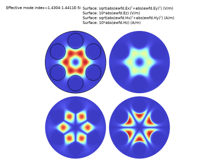
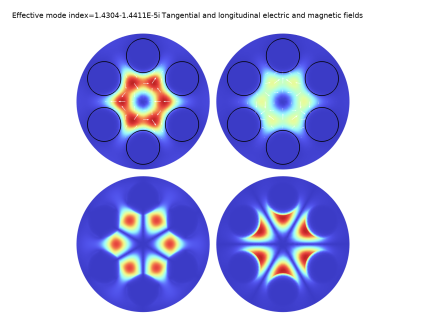
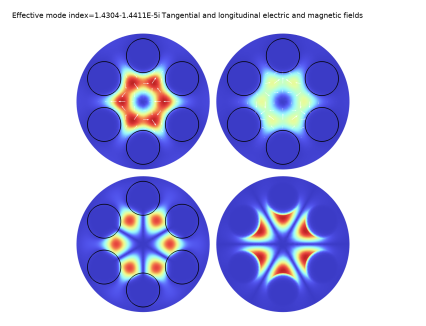
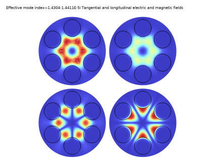
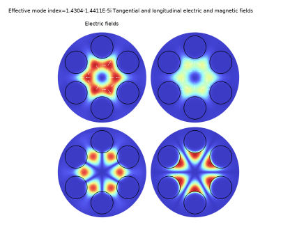
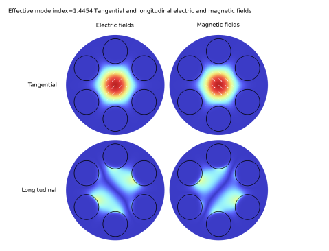
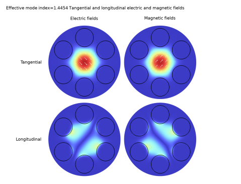
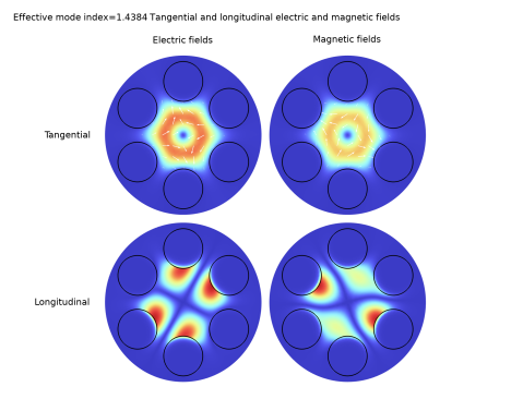
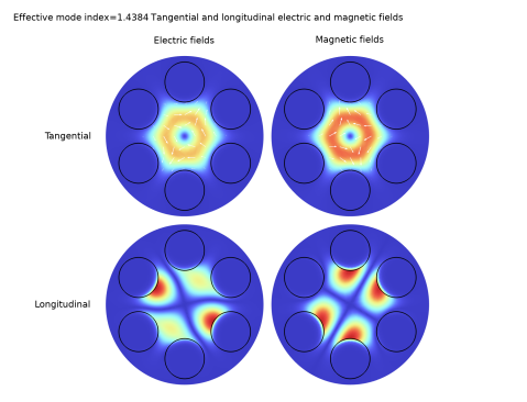
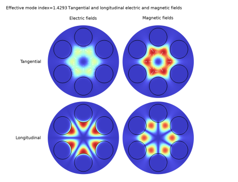
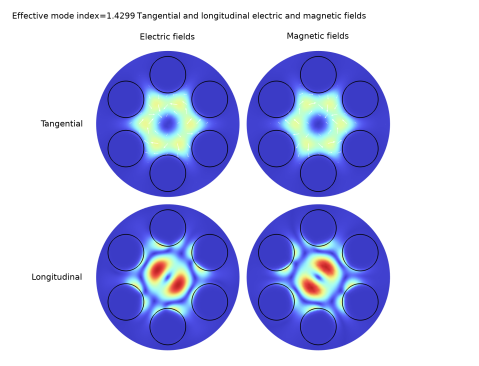
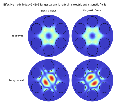
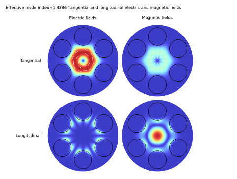
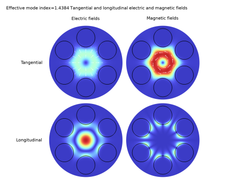
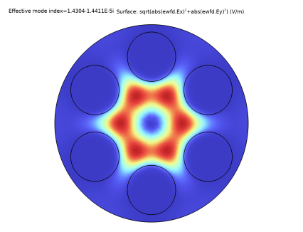
In the Expression text field, type sqrt(abs(ewfd.Ex)^2+abs(ewfd.Ey)^2). This represents the norm of the tangential electric field.
Surface 2
1
Right-click Results>Electric Field (ewfd)>Surface 1 and choose Duplicate.
2
In the Settings window for Surface, locate the Expression section.
3
In the Expression text field, type 10*abs(ewfd.Ez). This represents the norm of the longitudinal electric field. This component is scaled by a factor of ten, to make it visible when compared to the tangential electric field components.
4
Click to expand the Inherit Style section. From the Plot list, choose Surface 1.
Translation 1
1
Right-click Surface 2 and choose Translation.
2
In the Settings window for Translation, locate the Translation section.
3
In the y text field, type -2.1*rb.
4
Clear the Apply to dataset edges check box.
5
Click the  Zoom Extents button in the Graphics toolbar.
Surface 1, Surface 2
1
In the Model Builder window, under Results>Electric Field (ewfd), Ctrl-click to select Surface 1 and Surface 2.
2
Surface 3
1
In the Settings window for Surface, locate the Expression section.
2
In the Expression text field, type sqrt(abs(ewfd.Hx)^2+abs(ewfd.Hy)^2). This represents the norm of the tangential magnetic field.
Translation 1
1
Right-click Surface 3 and choose Translation.
2
In the Settings window for Translation, locate the Translation section.
3
In the x text field, type 2.1*rb.
4
Clear the Apply to dataset edges check box.
5
Click the  Zoom Extents button in the Graphics toolbar.
Surface 4
1
In the Model Builder window, expand the Results>Electric Field (ewfd)>Surface 4 node, then click Surface 4.
2
In the Settings window for Surface, locate the Expression section.
3
In the Expression text field, type 10*abs(ewfd.Hz). This represents the norm of the longitudinal magnetic field. Again, a scale factor of 10 is used here to make the longitudinal component visible when compared to the tangential components.
4
Locate the Inherit Style section. From the Plot list, choose Surface 3.
Translation 1
1
In the Model Builder window, click Translation 1.
2
In the Settings window for Translation, locate the Translation section.
3
In the x text field, type 2.1*rb.
Electric Field (ewfd)
1
In the Model Builder window, under Results click Electric Field (ewfd).
2
In the Settings window for 2D Plot Group, click to expand the Title section.
3
From the Title type list, choose Manual.
4
In the Title text area, type Tangential and longitudinal electric and magnetic fields.
Add arrow plots to visualize the polarization direction.
Arrow Surface 1
1
Right-click Electric Field (ewfd) and choose Arrow Surface.
2
In the Settings window for Arrow Surface, locate the Coloring and Style section.
3
From the Color list, choose White.
Translation 1
1
Right-click Arrow Surface 1 and choose Translation.
2
In the Settings window for Translation, locate the Translation section.
3
In the x text field, type 2.1*rb.
4
Clear the Apply to dataset edges check box.
Arrow Surface 2
1
In the Model Builder window, under Results>Electric Field (ewfd) right-click Arrow Surface 1 and choose Duplicate.
2
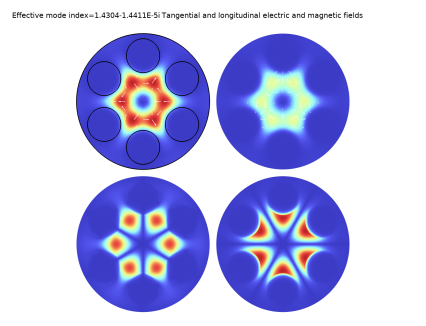
In the Settings window for Arrow Surface, click Replace Expression in the upper-right corner of the Expression section. From the menu, choose Component 1 (comp1)>Electromagnetic Waves, Frequency Domain>Electric>ewfd.Ex,ewfd.Ey - Electric field.
Translation 1
1
In the Model Builder window, expand the Arrow Surface 2 node.
2
Right-click Results>Electric Field (ewfd)>Arrow Surface 2>Translation 1 and choose Delete.
To clearly see the different polarization directions for the two degenerate modes with the highest effective indices, it helps here to change the phase of the solution to 45 degrees. Another option to see the different polarization directions would be to make an animation of one harmonic period.
Study 1/Solution 1 (sol1)
1
In the Model Builder window, expand the Results>Datasets node, then click Study 1/Solution 1 (sol1).
2
In the Settings window for Solution, locate the Solution section.
3
In the Solution at angle (phase) text field, type 45.
Arrow Surface 2
Electric Field (ewfd)
Now, remove the black edges and then add them back using line plots. This will make the location of the air holes more visible.
1
In the Model Builder window, click Electric Field (ewfd).
2
In the Settings window for 2D Plot Group, locate the Plot Settings section.
3
Clear the Plot dataset edges check box.
Line 1
1
Right-click Electric Field (ewfd) and choose Line.
2
In the Settings window for Line, locate the Coloring and Style section.
3
From the Coloring list, choose Uniform.
4
From the Color list, choose Black.
Selection 1
1
Right-click Line 1 and choose Selection.
2
In the Settings window for Selection, locate the Selection section.
3
From the Selection list, choose Air Hole Boundaries.
Line 2
In the Model Builder window, under Results>Electric Field (ewfd) right-click Line 1 and choose Duplicate.
Translation 1
1
In the Model Builder window, right-click Line 2 and choose Translation.
2
In the Settings window for Translation, locate the Translation section.
3
In the x text field, type 2.1*rb.
Line 1, Line 2
1
In the Model Builder window, under Results>Electric Field (ewfd), Ctrl-click to select Line 1 and Line 2.
2
Translation 1
1
In the Model Builder window, right-click Line 3 and choose Translation.
2
In the Settings window for Translation, locate the Translation section.
3
In the y text field, type -2.1*rb.
Translation 1
1
In the Model Builder window, expand the Results>Electric Field (ewfd)>Line 4 node, then click Translation 1.
2
In the Settings window for Translation, locate the Translation section.
3
In the y text field, type -2.1*rb.
Electric Field (ewfd)
Finally, add some informative annotations.
Annotation 1
1
In the Model Builder window, right-click Electric Field (ewfd) and choose Annotation.
2
In the Settings window for Annotation, locate the Annotation section.
3
In the Text text field, type Electric fields.
4
Locate the Position section. In the Y text field, type 1.2*rb.
5
Locate the Coloring and Style section. Clear the Show point check box.
6
From the Anchor point list, choose Center.
7
Click the  Zoom Extents button in the Graphics toolbar.
Annotation 2
1
Right-click Annotation 1 and choose Duplicate.
2
In the Settings window for Annotation, locate the Annotation section.
3
In the Text text field, type Magnetic fields.
4
Locate the Position section. In the X text field, type 2.1*rb.
Annotation 3
1
In the Model Builder window, under Results>Electric Field (ewfd) right-click Annotation 1 and choose Duplicate.
2
In the Settings window for Annotation, locate the Annotation section.
3
In the Text text field, type Tangential.
4
Locate the Position section. In the X text field, type -1.1*rb.
5
In the Y text field, type 0.
6
Locate the Coloring and Style section. From the Anchor point list, choose Middle right.
7
Click the  Zoom Extents button in the Graphics toolbar.
Annotation 4
1
Right-click Annotation 3 and choose Duplicate.
2
In the Settings window for Annotation, locate the Annotation section.
3
In the Text text field, type Longitudinal.
4
Locate the Position section. In the Y text field, type -2.1*rb.
Electric Field (ewfd)
1
In the Model Builder window, click Electric Field (ewfd).
2
In the Settings window for 2D Plot Group, locate the Title section.
3
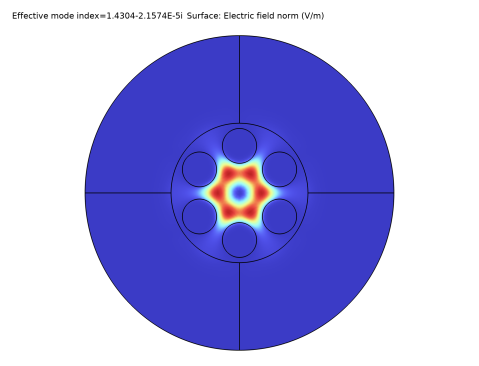
In the Parameter indicator text field, type Effective mode index=eval(ewfd.neff), to update the effective index in the title.
Now it is time to analyze the mode types, by stepping through the modes, starting with the mode with the largest effective index.
4
Click  Plot Last.
This is the first HE11-like mode. These modes are degenerate with a degeneracy of two. This mixed mode has both longitudinal electric and magnetic field components.
5
Click  Plot Previous.
This is the second degenerate HE11-like mode. The polarization is of course orthogonal to the first HE11-like mode.
6
Click  Plot Previous.
This is a TE01-like mode, where the field is almost rotationally invariant and polarized in the φ direction. As seen, the longitudinal electric field is very small, whereas the longitudinal magnetic field is non-negligible.
7
Click  Plot Previous.
This is the first degenerate HE21-like mode.
8
Click  Plot Previous.
This is the second degenerate HE21-like mode.
9
Click  Plot Previous.
This is a TM01-like mode, where the field is almost rotationally invariant and polarized in the radial direction. As seen, the longitudinal magnetic field is very small, whereas the longitudinal electric field is non-negligible.
10
Click  Plot Previous.
This is the first HE31-like mode.
11
Click  Plot Previous.
This is the first degenerate EH11-like mode.
12
Click  Plot Previous.
This is the second degenerate EH11-like mode.
13
Click  Plot Previous.
Finally, this is the second HE31-like mode.