PDF

Uncertainty Quantification of a Bracket
Introduction
This example demonstrates how to use the Uncertainty Quantification Module by running a series of uncertainty quantification studies for a steel bracket.
This type of bracket can be used to install an actuator that is mounted on a pin placed between the two holes in the bracket arms. The design objective is that the actuator’s horizontal misalignment should not be too large.
Figure 1: Bracket geometry with the quantity of interest, the misalignment angle, , indicated. The figure shows a different version of the bracket where fillets have been used (requires the Design Module).
Note: If you have access to the Design Module, a version using the 3D fillet functionality included with that product is also provided; see Uncertainty Quantification of a Bracket — Fillet Version. A few of the model parameters are slightly changed for the version with fillets but otherwise the instructions are identical.
Model Definition
The geometry is fully parameterized with parameters according to the table shown in Figure 2.
Figure 2: Geometry parameters.
The mesh is customized to have about two elements across the thickness of the material.
Figure 3: Meshed geometry.
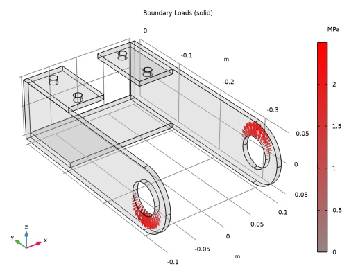
In this analysis, the mounting bolts are assumed to be fixed and securely bonded to the bracket. One of the arms is loaded upward and the other downward. The loads are applied as a pressure on the inner surfaces of the holes, and their intensity is P0 cos(α), where α is the angle from the direction of the load resultants.
Figure 4: Applied loads.
This force is assumed not to vary in the uncertainty quantification studies. Similarly, the material properties for a generic structural steel are assumed not to vary.
The misalignment angle is chosen as the quantity of interest (QoI). The design objective is that the actuator’s horizontal misalignment angle, , does not exceed 0.12 degree.1 The angle is defined as a global variable; for details, see the Modeling Instructions section.
The parameters to be varied are the geometric dimensions of the bracket.
The parameters that participate in the uncertainty quantification are all assumed to be normally distributed around their nominal values according to the table in Figure 5, which corresponds to the screening and sensitivity studies, as described later.
Figure 5: Input-parameter distributions used in screening and sensitivity studies.
The Uncertainty Quantification Studies
The Uncertainty Quantification Module provides four different study types:
-
-
-
-
-
-
-
-
-
For more information, see the Uncertainty Quantification Module User’s Guide.
Surrogate Models
To get statistical data based on a physics model you need to run a lot of simulations, varying the parameters of the inputs according to their probability distributions. For a 3D model, this might be computationally unfeasible. To get around this problem, the Uncertainty Quantification Module first builds up a so-called surrogate model that is used for sensitivity analysis, uncertainty propagation, and reliability analysis (but not for screening).
This process is typically adaptive and the surrogate model can approximate the original model to a high degree of accuracy (which can be modified by the user). The Uncertainty Quantification Module uses two different types of surrogate models:
-
-
Results and Discussion
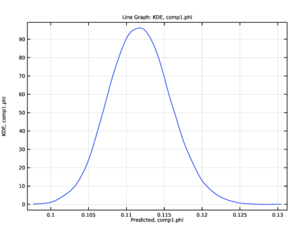
The uncertainty quantification study gives the kernel density estimation plot shown in Figure 6 with associated confidence interval information in the QOI confidence interval table, as shown in Figure 7.
Figure 6: Kernel density estimation.
Figure 7: QoI confidence interval.
The reliability analysis study shows that the probability for the misalignment angle not to exceed 0.12 degree is about 0.022 or 2.2%. This result is made available in the Probability for conditions table, as shown in Figure 8.
Figure 8: Probability for conditions.
Note that this value is sensitive to minute changes in the mesh and may vary a bit depending on the COMSOL Multiphysics version you are running.
It is now up to the designer to decide whether this is an acceptable level or risk or if a redesign and/or further studies are needed.
Application Library path: Uncertainty_Quantification_Module/Tutorials/bracket_uncertainty_quantification
Modeling Instructions
From the File menu, choose New.
New
In the New window, click  Model Wizard.
Model Wizard
1
In the Model Wizard window, click  3D.
2
In the Select Physics tree, select Structural Mechanics>Solid Mechanics (solid).
3
Click Add.
4
Click  Study.
5
In the Select Study tree, select General Studies>Stationary.
6
Geometry 1
1
In the Geometry toolbar, click Insert Sequence and choose Insert Sequence.
2
Browse to the model’s Application Libraries folder and double-click the file bracket_uncertainty_quantification_geom_sequence.mph.
3
In the Geometry toolbar, click  Build All.
Global Definitions
The geometry sequence already provided a set of geometry dimension parameters. Now define this additional set of parameters for the boundary load and mesh density.
Parameters 2
1
In the Home toolbar, click  Parameters and choose Add>Parameters.
2
In the Settings window for Parameters, locate the Parameters section.
3
Add Material
1
In the Home toolbar, click  Add Material to open the Add Material window.
2
Go to the Add Material window.
3
In the tree, select Built-in>Structural steel.
4
Click Add to Component in the window toolbar.
5
In the Home toolbar, click  Add Material to close the Add Material window.
Definitions
Next, define a series of Explicit selections to be used for the constraints and loads.
Bolt Holes
1
In the Model Builder window, expand the Component 1 (comp1)>Definitions node.
2
Right-click Definitions and choose Selections>Explicit.
3
In the Settings window for Explicit, locate the Input Entities section.
4
From the Geometric entity level list, choose Boundary.
5
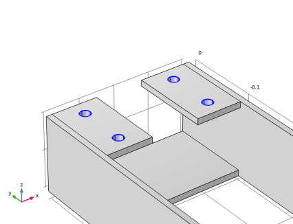
Select the Group by continuous tangent check box. This setting greatly facilitates the selection of curved surfaces. In this case use it to select the four bolt holes. It is sufficient to select one boundary per hole; the three other boundaries will be selected automatically.
6
In the Label text field, type Bolt Holes.
Left Pin Hole
1
In the Definitions toolbar, click  Explicit.
2
In the Settings window for Explicit, locate the Input Entities section.
3
From the Geometric entity level list, choose Boundary.
4
Select the Group by continuous tangent check box.
5
6
In the Label text field, type Left Pin Hole.
Right Pin Hole
1
In the Definitions toolbar, click  Explicit.
2
In the Settings window for Explicit, locate the Input Entities section.
3
From the Geometric entity level list, choose Boundary.
4
Select the Group by continuous tangent check box.
5
6
In the Label text field, type Right Pin Hole.
Pin Holes
1
In the Definitions toolbar, click  Union.
2
In the Settings window for Union, locate the Geometric Entity Level section.
3
From the Level list, choose Boundary.
4
Locate the Input Entities section. Under Selections to add, click  Add.
5
In the Add dialog box, in the Selections to add list, choose Left Pin Hole and Right Pin Hole.
6
7
In the Settings window for Union, type Pin Holes in the Label text field.
Define average operators that will be used for computing the average z-directional displacement of the pin holes.
Average 1 (aveop1)
1
In the Definitions toolbar, click  Nonlocal Couplings and choose Average.
2
In the Settings window for Average, locate the Source Selection section.
3
From the Geometric entity level list, choose Boundary.
4
From the Selection list, choose Left Pin Hole.
Average 2 (aveop2)
1
In the Definitions toolbar, click  Nonlocal Couplings and choose Average.
2
In the Settings window for Average, locate the Source Selection section.
3
From the Geometric entity level list, choose Boundary.
4
From the Selection list, choose Right Pin Hole.
Variables 1
1
Right-click Definitions and choose Variables.
Define the quantity of interest (QoI), the misalignment angle, as well as auxiliary variables for the pin hole z-coordinates.
2
In the Settings window for Variables, locate the Variables section.
3
The output from the atan() function has the unit radian, which is unitless. The conversion factor [1/deg] corresponds to multiplication by 180/pi for converting to degrees.
Now, define an analytic function load used to apply the spatially varying load on the pin holes.
Analytic 1 (an1)
1
In the Definitions toolbar, click  Analytic.
2
In the Settings window for Analytic, type load in the Function name text field.
3
Locate the Definition section. In the Expression text field, type F*cos(atan2(py,abs(px))).
4
In the Arguments text field, type F, py, px.
5
Locate the Units section. In the Function text field, type Pa.
6
Mesh 1
1
In the Model Builder window, under Component 1 (comp1) click Mesh 1.
2
In the Settings window for Mesh, locate the Sequence Type section.
3
From the list, choose User-controlled mesh.
Ensure that the mesh density is fine enough to resolve all the stress gradients reasonably well.
Size
1
In the Model Builder window, under Component 1 (comp1)>Mesh 1 click Size.
2
In the Settings window for Size, locate the Element Size section.
3
Click the Custom button.
4
Locate the Element Size Parameters section. In the Maximum element size text field, type hmax.
5
In the Minimum element size text field, type hmin.
6
Click  Build All.
Solid Mechanics (solid)
Apply fixed constraint boundary conditions on the bolt holes.
Fixed Constraint 1
1
In the Model Builder window, under Component 1 (comp1) right-click Solid Mechanics (solid) and choose Fixed Constraint.
2
In the Settings window for Fixed Constraint, locate the Boundary Selection section.
3
From the Selection list, choose Bolt Holes.
Next, apply the spatially varying load.
Boundary Load 1
1
In the Physics toolbar, click  Boundaries and choose Boundary Load.
2
In the Settings window for Boundary Load, locate the Coordinate System Selection section.
3
From the Coordinate system list, choose Boundary System 1 (sys1).
4
Locate the Force section. Specify the FA vector as
5
Locate the Boundary Selection section. From the Selection list, choose Pin Holes.
Study 1, Static
First, run a static analysis with no uncertainty quantification analysis.
1
In the Model Builder window, click Study 1.
2
In the Settings window for Study, type Study 1, Static in the Label text field.
3
In the Home toolbar, click  Compute.
Results
Volume 1
Now, let us assume that we are only interested in values up to 100 MPa.
1
In the Model Builder window, expand the Stress (solid) node, then click Volume 1.
2
In the Settings window for Volume, click to expand the Range section.
3
Locate the Expression section. From the Unit list, choose MPa.
4
In the Stress (solid) toolbar, click  Plot.
5
Locate the Range section. Select the Manual color range check box.
6
In the Maximum text field, type 100.
7
In the Stress (solid) toolbar, click  Plot.
Study 1, Static
In the Model Builder window, right-click Study 1, Static and choose Uncertainty Quantification>Add Uncertainty Quantification Study Using Study Reference.
Study 2, Screening
In the Settings window for Study, type Study 2, Screening in the Label text field.
Next, add a screening analysis to see which input parameters are most significantly impacting the misalignment angle (QoI). The screening study is added as a study reference which means it refers back to the already defined static study.
The parameters that participate in the uncertainty quantification are all assumed to be normally distributed around their nominal values, according to the instructions below. The mean and standard deviation, as well as the max and min limits are all defined in terms of their nominal parameters (from Global Definitions>Parameters).
Uncertainty Quantification
1
In the Model Builder window, under Study 2, Screening click Uncertainty Quantification.
2
In the Settings window for Uncertainty Quantification, locate the Quantities of Interest section.
3
4
5
Locate the Input Parameters section. Click  Add seven times.
6
7
8
From the Distribution list, choose Normal(μ,σ).
9
In the Mean text field, type ts.
10
In the Standard deviation text field, type 0.01*ts.
11
From the CDF-Lower list, choose Manual.
12
From the CDF-Upper list, choose Manual.
13
In the Lower bound text field, type 0.99*ts.
14
In the Upper bound text field, type 1.01*ts.
15
In the Unit text field, type m.
16
17
From the Distribution list, choose Normal(μ,σ).
18
In the Mean text field, type lp.
19
In the Standard deviation text field, type 0.01*lp.
20
From the CDF-Lower list, choose Manual.
21
From the CDF-Upper list, choose Manual.
22
In the Lower bound text field, type 0.95*lp.
23
In the Upper bound text field, type 1.05*lp.
24
In the Unit text field, type m.
25
26
From the Distribution list, choose Normal(μ,σ).
27
In the Mean text field, type ls.
28
In the Standard deviation text field, type 0.01*ls.
29
From the CDF-Lower list, choose Manual.
30
From the CDF-Upper list, choose Manual.
31
In the Lower bound text field, type 0.95*ls.
32
In the Upper bound text field, type 1.05*ls.
33
In the Unit text field, type m.
34
35
From the Distribution list, choose Normal(μ,σ).
36
In the Mean text field, type hm.
37
In the Standard deviation text field, type 0.01*hm.
38
From the CDF-Lower list, choose Manual.
39
From the CDF-Upper list, choose Manual.
40
In the Lower bound text field, type 0.95*hm.
41
In the Upper bound text field, type 1.05*hm.
42
In the Unit text field, type m.
43
44
From the Distribution list, choose Normal(μ,σ).
45
In the Mean text field, type wp.
46
In the Standard deviation text field, type 0.01*wp.
47
From the CDF-Lower list, choose Manual.
48
From the CDF-Upper list, choose Manual.
49
In the Lower bound text field, type 0.95*wp.
50
In the Upper bound text field, type 1.05*wp.
51
In the Unit text field, type m.
52
53
From the Distribution list, choose Normal(μ,σ).
54
In the Mean text field, type wf.
55
In the Standard deviation text field, type 0.01*wf.
56
From the CDF-Lower list, choose Manual.
57
From the CDF-Upper list, choose Manual.
58
In the Lower bound text field, type 0.95*wf.
59
In the Upper bound text field, type 1.05*wf.
60
In the Unit text field, type m.
61
62
From the Distribution list, choose Normal(μ,σ).
63
In the Mean text field, type r1.
64
In the Standard deviation text field, type 0.01*r1.
65
From the CDF-Lower list, choose Manual.
66
From the CDF-Upper list, choose Manual.
67
In the Lower bound text field, type 0.95*r1.
68
In the Upper bound text field, type 1.05*r1.
69
In the Unit text field, type m.
70
In the Home toolbar, click  Compute.
Results
MOAT, comp1.phi
1
Click the  Zoom Extents button in the Graphics toolbar.
The screening results indicate that the Side length (ls) and the Cross plate width (wp) parameters are the most influential on the quantity of interest. However, several of the other parameters also appear to be significant. A high value of the MOAT mean means that the parameter is significantly influencing the quantity of interest. A high value of the MOAT standard deviation means that the parameter is influential and that it is either interacting with other parameters and/or that it has a nonlinear influence.
Study 2, Screening
The next step is a sensitivity analysis. Use the results from the screening to decide which parameters to include in the sensitivity analysis. Sensitivity is more computationally demanding than screening and for this reason we would prefer to pick a subset of the parameters used for the screening study. However, in this example, we would like to learn as much as possible about the model and we pick all the available design parameters. We do not need to type all of the uncertainty quantification parameters again but we can define the new Uncertainty Quantification study for the sensitivity analysis by reusing the information in the screening study.
Uncertainty Quantification
Right-click Uncertainty Quantification and choose Add New Uncertainty Quantification Study For>Sensitivity Analysis.
Study 3, Sensitivity
1
In the Model Builder window, click Study 3.
2
In the Settings window for Study, type Study 3, Sensitivity in the Label text field.
Uncertainty Quantification
1
In the Model Builder window, under Study 3, Sensitivity click Uncertainty Quantification.
2
In the Settings window for Uncertainty Quantification, locate the Uncertainty Quantification Settings section.
3
From the Compute action list, choose Compute and analyze.
4
In the Home toolbar, click  Compute.
Results
Sobol Index, comp1.phi
The sensitivity analysis is based on the Sobol method, also known as variance-based sensitivity analysis. The result of the sensitivity analysis a set of Sobol indices and an associated Sobol table and Sobol plot. There are two different types of Sobol indices: first-order index and total index. The first-order index of a parameter shows the sensitivity by varying this parameter alone. The total index shows how much a parameter contributes to the overall sensitivity.
In this case, the first and total indices are equal, up to the computed accuracy, for all parameters which indicates very little or no interaction between the parameters. The Sobol plot indicates that the misalignment angle is most sensitive to the parameters Side length (ls) and Cross plate width (wp). This is consistent with the screening results.
For the final two studies, Uncertainty Propagation and Reliability Analysis, we will, for the purpose of faster demonstration, delete all parameters except for the dominant two, ls and wp. However, to get a conservative estimate of the uncertainties we should in principle include all parameters (see earlier comment).
Study 3, Sensitivity
Uncertainty Quantification
Right-click Uncertainty Quantification and choose Add New Uncertainty Quantification Study For>Uncertainty Propagation.
Study 4, Propagation
1
In the Model Builder window, click Study 4.
2
In the Settings window for Study, type Study 4, Propagation in the Label text field.
Uncertainty Quantification
1
In the Model Builder window, under Study 4, Propagation click Uncertainty Quantification.
2
In the Settings window for Uncertainty Quantification, locate the Input Parameters section.
3
4
Click  Delete.
5
Locate the Uncertainty Quantification Settings section. From the Compute action list, choose Compute and analyze. The default Compute action is Improve and analyze. This will reuse the previously computed uncertainty quantification results in order to speed up the computation. However, we are changing to Compute and analyze, which is slower, but gives a higher-fidelity result.
Uncertainty Quantification 3
In the Home toolbar, click  Compute.
Results
Kernel Density Estimation, comp1.phi
The uncertainty propagation study computes a so-called kernel density estimation or KDE. You can think of the KDE as a smooth form of a histogram showing an estimate of the probability density function of the quantity of interest, given the input parameters and their distributions. We can see from the QoI confidence interval table, shown earlier in the Results and Discussion section, that the mean is about 0.11 degree with a standard deviation of 0.004 degree. The KDE plot gives us this information graphically. From the values in the table we can also see that there appears to be some risk that the angle exceeds 0.12 degree.
To get a more accurate estimate of the risk for exceeding 0.12 degree, we will next run a reliability analysis.
Study 4, Propagation
Uncertainty Quantification
Right-click Uncertainty Quantification and choose Add New Uncertainty Quantification Study For>Reliability Analysis.
Study 5, Reliability
1
In the Model Builder window, click Study 5.
2
In the Settings window for Study, type Study 5, Reliability in the Label text field.
Uncertainty Quantification
1
In the Model Builder window, under Study 5, Reliability click Uncertainty Quantification.
2
In the Settings window for Uncertainty Quantification, locate the Quantities of Interest section.
3
Uncertainty Quantification 4
1
In the Home toolbar, click  Compute.
The reliability analysis performs a so-called importance sampling that refines the full model results near the threshold that we give for our quantity of interest. Recall that we are here asking for the probability that this angle exceeds 0.12 degree. The reliability analysis study gives us a table named Probability for condition having the value ~0.022. This means that with the given conditions, there is a ~2.2% risk of the misalignment angle to exceed 0.12 degree.
As a final step, we can also produce a response surface of pairs of input parameters, in this case the Side length (ls) and the Cross plate width (wp) .
Uncertainty Quantification
1
In the Model Builder window, under Study 5, Reliability click Uncertainty Quantification.
2
Locate the Surrogate-Based Response Surface section. Click Response Surface in the upper-right corner of the section.
Results
Response surface
Click the  Zoom Extents button in the Graphics toolbar.
 

1
The absence of fillets makes the bracket slightly less stiff, so this threshold value needs to be increased by about 20% compared to the value used in the fillet version of the model.