
|
|
|
|
•
|
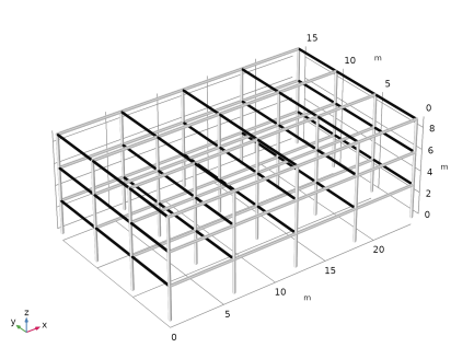
Number of columns in the X direction: 5
|
|
•
|
|
•
|
Number of columns in the Y direction: 4
|
|
•
|
|
•
|
Floor height: 3 m
|
|
•
|
Columns: Box 300-by-200 mm with wall thickness 10 mm. The stiff direction is along the global X-axis.
|
|
•
|
Horizontal beams in the X direction: HEA 260.
|
|
•
|
Horizontal beams in the Y direction: HEA 220.
|
|
•
|
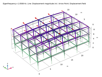
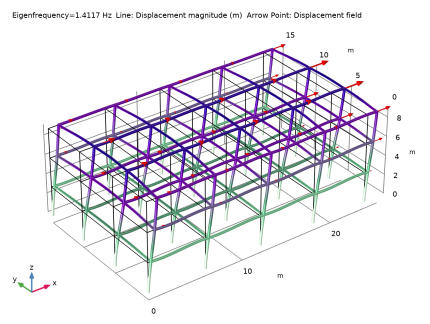
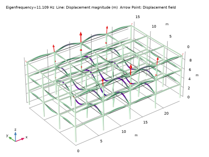
A split is made between periodic and rigid modes, using the Gupta method. Modes with higher natural frequencies are called rigid. The highest frequency at which the modes are fully periodic is set to 10 Hz, and the lowest frequency where the modes are fully in phase with each other is set to 20 Hz.
|
|
1
|
|
2
|
|
3
|
Click Add.
|
|
4
|
Click
|
|
5
|
|
6
|
Click
|
|
1
|
|
2
|
|
3
|
|
4
|
Browse to the model’s Application Libraries folder and double-click the file building_response_spectrum_parameters.txt.
|
|
1
|
|
2
|
|
3
|
|
4
|
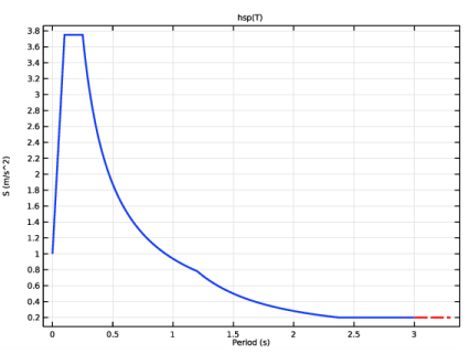
Browse to the model’s Application Libraries folder and double-click the file building_response_spectrum_horspec_parameters.txt.
|
|
1
|
|
2
|
|
3
|
|
4
|
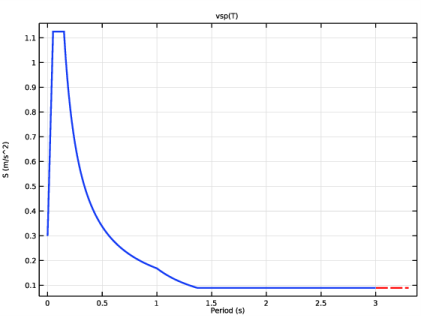
Browse to the model’s Application Libraries folder and double-click the file building_response_spectrum_vertspec_parameters.txt.
|
|
1
|
|
2
|
|
3
|
|
4
|
|
5
|
|
6
|
Browse to the model’s Application Libraries folder and double-click the file building_response_spectrum_horspec_function.txt.
|
|
7
|
|
1
|
In the Settings window for 1D Plot Group, type Horizontal Pseudoacceleration Spectrum in the Label text field.
|
|
2
|
|
3
|
|
4
|
|
1
|
In the Model Builder window, expand the Horizontal Pseudoacceleration Spectrum node, then click Function 1.
|
|
2
|
|
3
|
|
4
|
|
5
|
|
1
|
|
2
|
|
3
|
|
4
|
|
5
|
|
6
|
Browse to the model’s Application Libraries folder and double-click the file building_response_spectrum_vertspec_function.txt.
|
|
7
|
|
1
|
In the Settings window for 1D Plot Group, type Vertical Pseudoacceleration Spectrum in the Label text field.
|
|
2
|
|
3
|
|
4
|
|
1
|
In the Model Builder window, expand the Vertical Pseudoacceleration Spectrum node, then click Function 1.
|
|
2
|
|
3
|
|
4
|
|
5
|
|
1
|
In the Model Builder window, under Results, Ctrl-click to select Horizontal Pseudoacceleration Spectrum and Vertical Pseudoacceleration Spectrum.
|
|
2
|
Right-click and choose Group.
|
|
1
|
|
2
|
|
1
|
|
2
|
|
3
|
Locate the Coordinates section. In the table, enter the following settings:
|
|
4
|
Locate the Selections of Resulting Entities section. Find the Cumulative selection subsection. Click New.
|
|
5
|
|
6
|
Click OK.
|
|
1
|
|
2
|
Select the object pol1 only.
|
|
3
|
|
4
|
|
5
|
|
6
|
|
7
|
|
8
|
|
9
|
|
10
|
Locate the Selections of Resulting Entities section. Find the Cumulative selection subsection. From the Contribute to list, choose Columns.
|
|
11
|
|
12
|
|
1
|
|
2
|
|
3
|
Locate the Coordinates section. In the table, enter the following settings:
|
|
4
|
Locate the Selections of Resulting Entities section. Find the Cumulative selection subsection. Click New.
|
|
5
|
|
6
|
Click OK.
|
|
1
|
In the Model Builder window, under Component 1 (comp1)>Geometry 1 right-click Array 1 (arr1) and choose Duplicate.
|
|
2
|
|
3
|
|
4
|
|
5
|
Locate the Selections of Resulting Entities section. Find the Cumulative selection subsection. From the Contribute to list, choose Horizontal X.
|
|
6
|
|
7
|
|
1
|
|
2
|
|
3
|
Locate the Coordinates section. In the table, enter the following settings:
|
|
4
|
Locate the Selections of Resulting Entities section. Find the Cumulative selection subsection. Click New.
|
|
5
|
|
6
|
Click OK.
|
|
1
|
In the Model Builder window, under Component 1 (comp1)>Geometry 1 right-click Array 2 (arr2) and choose Duplicate.
|
|
2
|
|
3
|
|
4
|
|
5
|
|
6
|
|
7
|
Locate the Selections of Resulting Entities section. Find the Cumulative selection subsection. From the Contribute to list, choose Horizontal Y.
|
|
8
|
|
1
|
|
2
|
|
3
|
|
4
|
|
1
|
|
2
|
In the Settings window for Cross-Section Data, type Cross Section Data - Columns in the Label text field.
|
|
3
|
|
4
|
|
5
|
|
6
|
|
7
|
|
8
|
|
1
|
|
2
|
|
3
|
|
4
|
Specify the V vector as
|
|
1
|
|
2
|
In the Settings window for Cross-Section Data, type Cross Section: Horizontal X (HEA260) in the Label text field.
|
|
3
|
|
4
|
|
5
|
|
6
|
|
7
|
|
8
|
|
9
|
|
1
|
In the Model Builder window, expand the Cross Section: Horizontal X (HEA260) node, then click Section Orientation 1.
|
|
2
|
|
3
|
|
4
|
Specify the V vector as
|
|
1
|
|
2
|
In the Settings window for Cross-Section Data, type Cross Section: Horizontal Y (HEA220) in the Label text field.
|
|
3
|
|
4
|
|
5
|
|
6
|
|
7
|
|
1
|
|
2
|
|
3
|
|
4
|
|
1
|
|
2
|
|
3
|
|
1
|
|
2
|
|
3
|
|
1
|
|
2
|
|
3
|
|
4
|
|
5
|
|
1
|
|
2
|
|
3
|
|
1
|
|
2
|
|
1
|
|
2
|
|
3
|
|
4
|
|
5
|
|
1
|
|
2
|
|
1
|
|
2
|
|
3
|
|
1
|
|
2
|
|
3
|
|
1
|
|
2
|
|
3
|
|
4
|
|
1
|
In the Model Builder window, under Results, Ctrl-click to select Stress (beam) and Beam Orientation (beam).
|
|
2
|
Right-click and choose Group.
|
|
1
|
|
2
|
|
1
|
|
2
|
|
3
|
|
4
|
|
5
|
|
6
|
|
7
|
|
1
|
|
2
|
|
3
|
Locate the Combine Solutions Settings section. From the Solution operation list, choose Remove solutions.
|
|
4
|
|
5
|
In the Excluded if text field, type (comp1.rsp1.mEffLX<comp1.rsp1.mass*massTol)&&(comp1.rsp1.mEffLY<comp1.rsp1.mass*massTol)&&(comp1.rsp1.mEffLZ<comp1.rsp1.mass*massTol).
|
|
6
|
|
7
|
|
8
|
|
9
|
|
10
|
|
1
|
|
2
|
|
3
|
|
4
|
Click Replace Expression in the upper-right corner of the Expressions section. From the menu, choose Component 1 (comp1)>Definitions>Response Spectrum 1>Effective modal mass>rsp1.mEffLX - Effective modal mass, X-translation - kg.
|
|
5
|
Locate the Expressions section. In the table, enter the following settings:
|
|
6
|
|
7
|
|
8
|
Click
|
|
1
|
|
2
|
|
3
|
|
4
|
|
5
|
Click Replace Expression in the upper-right corner of the Expressions section. From the menu, choose Component 1 (comp1)>Definitions>Response Spectrum 1>rsp1.mass - Mass - kg.
|
|
6
|
Click
|
|
1
|
|
2
|
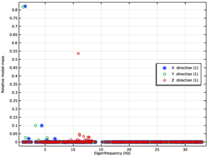
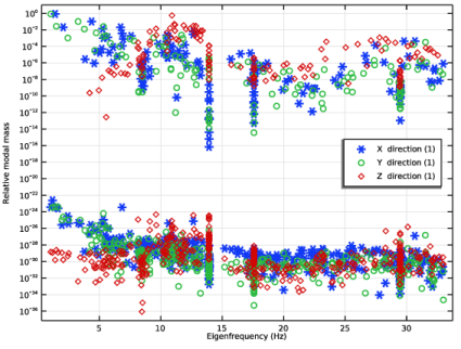
In the Settings window for Global Evaluation, type Relative Modal Mass Contribution in the Label text field.
|
|
3
|
Locate the Expressions section. In the table, enter the following settings:
|
|
4
|
Locate the Data section. From the Dataset list, choose Study: Eigenfrequency/Solution Store 1 (sol3).
|
|
5
|
Click
|
|
1
|
Go to the Table window.
|
|
2
|
|
1
|
|
2
|
|
3
|
|
4
|
|
5
|
|
1
|
|
2
|
|
3
|
|
4
|
|
5
|
|
6
|
|
7
|
|
8
|
|
1
|
|
2
|
|
3
|
|
1
|
|
2
|
|
1
|
|
2
|
|
3
|
|
4
|
|
5
|
|
6
|
|
1
|
In the Model Builder window, under Results, Ctrl-click to select Mode Shape (beam) and Relative Modal Mass.
|
|
2
|
Right-click and choose Group.
|
|
1
|
|
2
|
|
1
|
|
2
|
|
3
|
|
4
|
|
5
|
|
6
|
|
7
|
|
1
|
|
2
|
|
1
|
|
2
|
|
3
|
|
4
|
|
5
|
|
1
|
|
2
|
|
3
|
|
4
|
|
1
|
|
2
|
|
1
|
|
2
|
|
3
|
|
4
|
|
5
|
|
6
|
|
7
|
Click OK.
|
|
8
|
|
1
|
In the Model Builder window, expand the Component 1 (comp1)>Definitions node, then click Response Spectrum 1 (rsp1).
|
|
2
|
In the Settings window for Response Spectrum, click in the upper-right corner of the Response Spectrum section. Locate the Response Spectrum section. Click Create Missing Mass Correction Study in the upper-right corner of the section.
|
|
1
|
In the Model Builder window, expand the Study: Missing Mass Load Cases node, then click Step 4: Missing Mass Static Load Cases.
|
|
2
|
|
3
|
|
4
|
|
5
|
Right-click and choose Disable.
|
|
6
|
|
1
|
In the Model Builder window, under Results>Datasets right-click Response Spectrum 3D 1 and choose Duplicate.
|
|
2
|
|
3
|
|
4
|
|
5
|
|
6
|
|
7
|
|
8
|
Locate the Data section. From the Missing mass load cases dataset list, choose Study: Missing Mass Load Cases/Solution 4 (sol4).
|
|
1
|
In the Model Builder window, under Results, Ctrl-click to select Stress, CQC Method and Displacement, CQC Method.
|
|
2
|
Right-click and choose Duplicate.
|
|
1
|
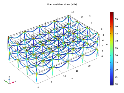
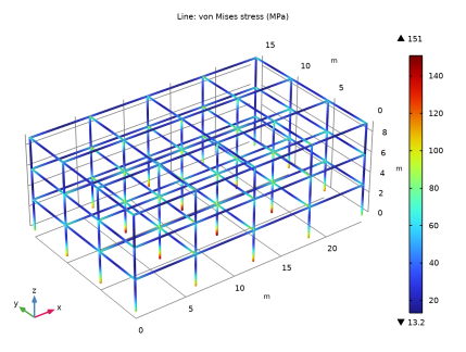
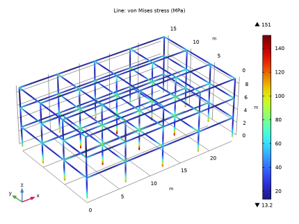
In the Settings window for 3D Plot Group, type Stress, CQC Method with Missing Mass Correction in the Label text field.
|
|
2
|
|
3
|
|
4
|
Click
|
|
1
|
|
2
|
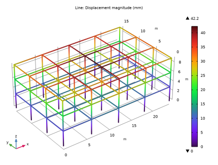
In the Settings window for 3D Plot Group, type Displacement, CQC Method with Missing Mass Correction in the Label text field.
|
|
3
|
|
4
|