You are viewing the documentation for an older COMSOL version. The latest version is available here.
PDF

Annular Ultraviolet Reactor
Introduction
In this example, the fluence rate distribution is computed in a simple ultraviolet (UV) water purification reactor. The fluence rate is the amount of radiation that a tiny spherical detector would be exposed to at any point in space, divided by the cross sectional area of such a detector. Fluence rate is a key figure of merit in the evaluation of UV water purification systems because it determines the amount of radiation that bacteria and other pathogens will absorb as they are carried by water flowing past an ultraviolet lamp.
In this example, only the fluence rate will be considered. To also consider how the water flows through the reactor and how the UV dose is accumulated for particles carried by the flow, see the example Annular Ultraviolet Reactor with Particle Tracing: Ray_Optics_Module/Ultraviolet_Sterilization/annular_ultraviolet_reactor_particle.
Model Definition
The model geometry consists of the annular region between a cylindrical UV lamp and the cylindrical reactor that surrounds it. In practice, this reactor would be connected to inlet and outlet tubes so that water can flow past the UV lamp, but in this model only the fluence rate in the immediate vicinity of the lamp is considered.
Ultraviolet Lamp Model
The surface of the lamp is treated as a diffuse (Lambertian) emitter using the Release from Boundary node. Rays are released at the lamp surface with uniform spatial density, and the initial direction of each ray is sampled according to the cosine law. The total power of the lamp is specified; in this example the power distribution over the lamp surface area is assumed to be uniform, although it is also possible to define a weighting factor.
As rays propagate through the water, away from the lamp surface, the power of each ray is attenuated based on the internal transmittance of the water, which in this example is taken to be 70% per centimeter of propagation. For distilled water, the internal transmittance of germicidal UV radiation is approximately 98%, so the value of 70% used here could represent that the water is less pure.
As rays propagate through the water, the volumetric fluence rate is computed using the dedicated Fluence Rate Calculation node. To obtain an accurate distribution of the fluence rate, it is important to release a sufficiently large number of rays and to use a sufficiently fine mesh in the domain. In this example, 100,000 rays were released in order to balance accuracy with solution time and file size considerations, but in some publications the number of rays could be orders of magnitude greater (Ref. 1).
Rather than releasing rays diffusely at the lamp surface, a possible extension of this model would be to release rays from within the volume of the lamp, or to release them from a narrower surface inside the lamp, which could represent an arc that produces the UV radiation. At the lamp surface, then, the light could be refracted into the water domain according to Snell’s law and the Fresnel equations.
The dependence of the fluence rate on the other boundary conditions in the model is also considered. In the first study, the walls are assumed to be perfect absorbers of UV radiation, using the Wall node. In the second study, the walls are treated as perfect reflectors using the Mirror node. Eventually, due to the attenuation within the water domain, each ray will make negligible contributions to the fluence rate even as it continues to be reflected at the outer surfaces of the reactor.
Results and Discussion
The fluence rate distribution in a slice of the reactor is shown in Figure 1. The fluence rate is greatest in the immediate vicinity of the lamp and it falls off at a greater distance.
Figure 1: Fluence rate distribution in a cross section of the annular UV reactor, assuming totally absorbing walls.
A 1D plot of the radial fluence rate distribution is shown in Figure 2. The very jagged plot is the actual computed value of the fluence rate along a Cut Line 3D dataset through the domain. The individual segments of this plot are flat with jump discontinuities between them because the Fluence Rate Calculation node uses constant shape functions to define the fluence rate in each mesh element that the cut line intersects.
To make the plot less mesh-dependent, a finer mesh could be used, together with a significantly increased number of rays. This example uses only 100,000 rays, whereas in Ref. 1 most values are in the tens of millions of rays. In exchange for using a larger number of rays, the solution time and the memory footprint of the model would increase. Refining the mesh while keeping the number of rays fixed is not recommended because some small mesh elements will not be hit by any ray, and they will erroneously report zero fluence rate.
A low-cost alternative approach to smoothing out the fluence rate distribution is to exploit the axial symmetry of the geometry. At any point outside the lamp, the exact value of the fluence rate can be replaced with the average value over all points having the same radial and axial coordinates,
In this example the average over all azimuthal angles is performed using a General Projection coupling. In the Source Map settings for this coupling, the expressions for ρ, z, and φ are entered (in terms of the Cartesian coordinates), while in the Destination Map section only ρ and z are entered. As a result, the expression genproj1(expr) integrates the expression expr along a ring centered at the z-axis.
Since the UV transmittance is 70% per centimeter in this model, and even the shortest distance from lamp to the exterior cylindrical boundaries is 4 cm, the ray power is reduced by at least 75% for rays that reach these outer boundaries (because 0.74 is approximately 0.25). Nevertheless, by applying a Mirror boundary condition, the reflected light can still notably affect the fluence rate near the outer walls. The difference in azimuthally averaged fluence rate distribution between absorbing and reflecting walls is shown in Figure 3. While the two curves appear to be very close together, at the maximum radial coordinate the difference between them is a significant fraction of the fluence rate magnitude. Therefore, the effect of reflection can significantly alter the accumulated dose for particles that flow through the reactor at the maximum possible radial coordinate.
Figure 2: Comparison of the computed radial fluence rate distribution with the azimuthally averaged value and a simplified analytic solution.
Figure 3: Comparison of the fluence rate distribution for absorbing and reflecting walls.
Reference
1. Y.M. Ahmed, M. Jongewaard, M. Li, and E.R. Blatchley III, “Ray Tracing for Fluence Rate Simulations in Ultraviolet Photoreactors,” Environ. Sci. Technol., vol. 52, no. 8, pp. 4738–4745, 2018.
Application Library path: Ray_Optics_Module/Ultraviolet_Sterilization/annular_ultraviolet_reactor
Modeling Instructions
From the File menu, choose New.
New
In the New window, click  Model Wizard.
Model Wizard
1
In the Model Wizard window, click  3D.
2
In the Select Physics tree, select Optics>Ray Optics>Geometrical Optics (gop).
3
Click Add.
4
Click  Study.
5
In the Select Study tree, select Preset Studies for Selected Physics Interfaces>Ray Tracing.
6
Global Definitions
Parameters 1
1
In the Model Builder window, under Global Definitions click Parameters 1.
2
In the Settings window for Parameters, locate the Parameters section.
3
Geometry 1
Reactor
1
In the Geometry toolbar, click  Cylinder.
2
In the Settings window for Cylinder, type Reactor in the Label text field.
3
Locate the Size and Shape section. In the Radius text field, type r_reac.
4
In the Height text field, type L_reac.
Lamp
1
In the Geometry toolbar, click  Cylinder.
2
In the Settings window for Cylinder, type Lamp in the Label text field.
3
Locate the Size and Shape section. In the Radius text field, type r_lamp.
4
In the Height text field, type L_lamp.
5
Locate the Position section. In the z text field, type d_lamp.
Difference 1 (dif1)
1
In the Geometry toolbar, click  Booleans and Partitions and choose Difference.
2
3
In the Settings window for Difference, locate the Difference section.
4
Find the Objects to subtract subsection. Click to select the  Activate Selection toggle button.
5
6
In the Geometry toolbar, click  Build All.
Add a General Projection coupling to be used in results processing.
Definitions
General Projection 1 (genproj1)
1
In the Definitions toolbar, click  Nonlocal Couplings and choose General Projection.
2
3
In the Settings window for General Projection, locate the Source Map section.
4
In the x-expression text field, type sqrt(x^2+y^2).
5
In the y-expression text field, type z.
6
In the z-expression text field, type atan2(y,x).
7
Locate the Destination Map section. In the x-expression text field, type sqrt(x^2+y^2).
8
In the y-expression text field, type z.
The above expressions represent a conversion from Cartesian to cylindrical polar coordinates. For any point (r, z) in the geometry, the input argument to this projection coupling will be integrated for all azimuthal angles φ from 0 to π.
Geometrical Optics (gop)
1
In the Model Builder window, under Component 1 (comp1) click Geometrical Optics (gop).
2
In the Settings window for Geometrical Optics, locate the Ray Release and Propagation section.
3
In the Maximum number of secondary rays text field, type 0.
4
Select the Only store accumulated variables in solution check box.
5
Locate the Intensity Computation section. From the Intensity computation list, choose Compute power.
Ray Properties 1
1
In the Model Builder window, under Component 1 (comp1)>Geometrical Optics (gop) click Ray Properties 1.
2
In the Settings window for Ray Properties, locate the Ray Properties section.
3
In the λ0 text field, type 254[nm]. A low-pressure mercury vapor lamp would emit most of its UV radiation at this wavelength (Ref. 1).
Medium Properties 1
1
In the Model Builder window, click Medium Properties 1.
2
In the Settings window for Medium Properties, locate the Medium Properties section.
3
From the n list, choose User defined. In the associated text field, type 1.38. This is approximately the refractive index of water at 254 nm (Ref. 1).
4
From the Optical attenuation model list, choose Internal transmittance, 10 mm sample thickness.
5
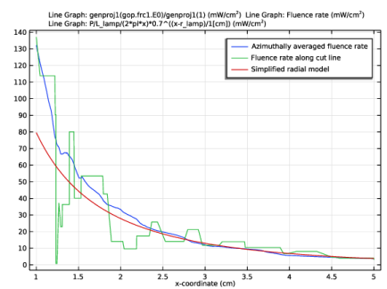
From the τi,10 list, choose User defined. In the associated text field, type 0.7. Different values of the internal transmittance of water can be used here, depending on the clarity of the water. For pure water, the internal transmittance of germicidal UV radiation is about 0.98 per centimeter (Ref. 1). The value of 0.7 shown here indicates that the water is less clear.
Release from Boundary 1
1
In the Physics toolbar, click  Boundaries and choose Release from Boundary.
2
3
In the Settings window for Release from Boundary, locate the Initial Position section.
4
From the Initial position list, choose Density.
5
In the N text field, type 100000.
6
Locate the Ray Direction Vector section. From the Ray direction vector list, choose Lambertian.
7
Select the Specify tangential and normal vector components check box.
8
In the Nw text field, type 1.
9
Specify the r vector as
10
From the Sampling from distribution list, choose Random.
These settings will cause rays to be released from the lamp surface with uniform spatial density, with a distribution of initial directions following the cosine law with respect to the surface normal at each release position. To ensure that the surface normal points in the outward direction rather than the inward direction, look for the arrows in the Graphics window.
11
Locate the Total Source Power section. In the Psrc text field, type P.
Fluence Rate Calculation 1
1
In the Physics toolbar, click  Domains and choose Fluence Rate Calculation.
2
Wall 1
1
In the Physics toolbar, click  Boundaries and choose Wall.
2
In the Settings window for Wall, locate the Boundary Selection section.
3
From the Selection list, choose All boundaries.
Add a Mirror boundary condition. This will be disabled in the first study, so that all of the exterior boundaries absorb the outgoing UV radiation. Then the Mirror boundary condition will be enabled in a second study to predict the effects of reflection on the fluence rate distribution.
Mirror 1
1
In the Physics toolbar, click  Boundaries and choose Mirror.
2
In this example a Free Tetrahedral mesh is used. To get higher resolution of the radial dependence of the fluence rate, a structured mesh could be created, although this may require the addition of mesh control surfaces to the geometry sequence.
Mesh 1
1
In the Model Builder window, under Component 1 (comp1) click Mesh 1.
2
In the Settings window for Mesh, locate the Physics-Controlled Mesh section.
3
From the Element size list, choose Extra fine.
4
Click  Build All.
Study 1: Absorbing Walls
1
In the Model Builder window, click Study 1.
2
In the Settings window for Study, type Study 1: Absorbing Walls in the Label text field.
Step 1: Ray Tracing
1
In the Model Builder window, under Study 1: Absorbing Walls click Step 1: Ray Tracing.
2
In the Settings window for Ray Tracing, locate the Study Settings section.
3
From the Time-step specification list, choose Specify maximum path length.
4
In the Lengths text field, type 0 0.2.
5
Locate the Physics and Variables Selection section. Select the Modify model configuration for study step check box.
6
In the tree, select Component 1 (comp1)>Geometrical Optics (gop)>Mirror 1.
7
8
In the Home toolbar, click  Compute.
Results
Fluence Rate Slice Plot
1
In the Home toolbar, click  Add Plot Group and choose 3D Plot Group.
2
In the Settings window for 3D Plot Group, type Fluence Rate Slice Plot in the Label text field.
Slice 1
1
In the Fluence Rate Slice Plot toolbar, click  Slice.
2
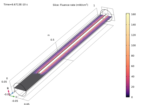
In the Settings window for Slice, click Replace Expression in the upper-right corner of the Expression section. From the menu, choose Component 1 (comp1)>Geometrical Optics>Heating and losses>gop.frc1.E0 - Fluence rate - W/m².
3
Locate the Expression section. In the Unit field, type mW/cm^2.
4
Locate the Plane Data section. In the Planes text field, type 1.
5
Click to expand the Quality section. From the Resolution list, choose No refinement.
6
Locate the Coloring and Style section. Click  Change Color Table.
7
In the Color Table dialog box, select Thermal>Magma in the tree.
8
9
In the Settings window for Slice, locate the Coloring and Style section.
10
From the Color table transformation list, choose Nonlinear.
11
Set the Color calibration parameter value to -1.5.
12
In the Fluence Rate Slice Plot toolbar, click  Plot. Compare the resulting plot to Figure 1.
Cut Line 3D 1
1
In the Results toolbar, click  Cut Line 3D.
2
In the Settings window for Cut Line 3D, locate the Line Data section.
3
In row Point 1, set X to r_lamp.
4
In row Point 1, set Z to mid_lamp.
5
In row Point 2, set X to r_reac.
6
In row Point 2, set Z to mid_lamp.
7
Fluence Rate Radial Distribution
1
In the Results toolbar, click  1D Plot Group.
2
In the Settings window for 1D Plot Group, type Fluence Rate Radial Distribution in the Label text field.
3
Locate the Data section. From the Dataset list, choose Cut Line 3D 1.
4
From the Time selection list, choose Last.
Line Graph 1
1
In the Fluence Rate Radial Distribution toolbar, click  Line Graph.
2
In the Settings window for Line Graph, locate the y-Axis Data section.
3
In the Expression text field, type genproj1(gop.frc1.E0)/genproj1(1).
4
In the Unit field, type mW/cm^2.
5
Locate the x-Axis Data section. From the Parameter list, choose Expression.
6
In the Expression text field, type x.
7
From the Unit list, choose cm.
8
Click to expand the Legends section. Select the Show legends check box.
9
From the Legends list, choose Manual.
10
Line Graph 2
1
Right-click Line Graph 1 and choose Duplicate.
2
In the Settings window for Line Graph, locate the y-Axis Data section.
3
In the Expression text field, type gop.frc1.E0.
4
Locate the Legends section. In the table, enter the following settings:
Line Graph 3
1
Right-click Line Graph 2 and choose Duplicate.
2
In the Settings window for Line Graph, locate the y-Axis Data section.
3
In the Expression text field, type P/L_lamp/(2*pi*x)*0.7^((x-r_lamp)/1[cm]).
4
Locate the Legends section. In the table, enter the following settings:
5
In the Fluence Rate Radial Distribution toolbar, click  Plot. Compare the resulting plot to Figure 2.
Add Study
1
In the Home toolbar, click  Add Study to open the Add Study window.
2
Go to the Add Study window.
3
Find the Studies subsection. In the Select Study tree, select Preset Studies for Selected Physics Interfaces>Ray Tracing.
4
Click Add Study in the window toolbar.
5
In the Home toolbar, click  Add Study to close the Add Study window.
Study 2
Step 1: Ray Tracing
1
In the Settings window for Ray Tracing, locate the Study Settings section.
2
From the Time-step specification list, choose Specify maximum path length.
3
In the Lengths text field, type 0 0.2.
4
In the Model Builder window, click Study 2.
5
In the Settings window for Study, type Study 2: Reflecting Walls in the Label text field.
6
In the Home toolbar, click  Compute.
Results
Cut Line 3D 2
1
In the Model Builder window, under Results>Datasets right-click Cut Line 3D 1 and choose Duplicate.
2
In the Settings window for Cut Line 3D, locate the Data section.
3
From the Dataset list, choose Study 2: Reflecting Walls/Solution 2 (sol2).
Absorbing vs Reflecting Reactor
1
In the Model Builder window, right-click Fluence Rate Radial Distribution and choose Duplicate.
2
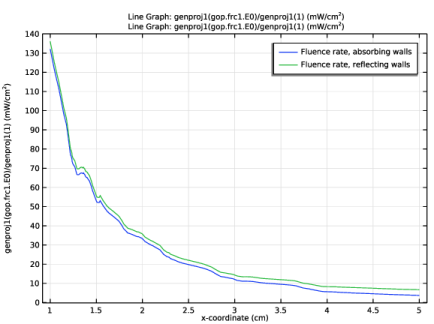
In the Settings window for 1D Plot Group, type Absorbing vs Reflecting Reactor in the Label text field.
3
In the Model Builder window, expand the Absorbing vs Reflecting Reactor node.
Line Graph 2, Line Graph 3
1
In the Model Builder window, under Results>Absorbing vs Reflecting Reactor, Ctrl-click to select Line Graph 2 and Line Graph 3.
2
Line Graph 1
1
In the Model Builder window, under Results>Absorbing vs Reflecting Reactor click Line Graph 1.
2
In the Settings window for Line Graph, locate the Legends section.
3
Line Graph 2
1
Right-click Results>Absorbing vs Reflecting Reactor>Line Graph 1 and choose Duplicate.
2
In the Settings window for Line Graph, locate the Data section.
3
From the Dataset list, choose Cut Line 3D 2.
4
From the Time selection list, choose Last.
5
Locate the Legends section. In the table, enter the following settings:
6
In the Absorbing vs Reflecting Reactor toolbar, click  Plot. Compare the resulting plot to Figure 3.