
|
|
|
|
•
|
|
•
|
dp (SI unit: m) is the particle diameter, and
|
|
•
|
μ (SI unit: Pa s) is the dynamic viscosity of the surrounding fluid.
|
|
1
|
|
2
|
|
3
|
Click Add.
|
|
4
|
In the Select Physics tree, select Fluid Flow>Single-Phase Flow>Turbulent Flow>Turbulent Flow, k-ε (spf).
|
|
5
|
Click Add.
|
|
6
|
In the Select Physics tree, select Fluid Flow>Particle Tracing>Particle Tracing for Fluid Flow (fpt).
|
|
7
|
Click Add.
|
|
8
|
Click
|
|
9
|
In the Select Study tree, select Preset Studies for Selected Physics Interfaces>Geometrical Optics>Ray Tracing.
|
|
10
|
Click
|
|
1
|
|
2
|
|
1
|
|
2
|
|
3
|
|
4
|
|
1
|
|
2
|
|
3
|
|
4
|
|
5
|
|
6
|
|
1
|
|
2
|
|
3
|
|
4
|
|
5
|
|
6
|
|
1
|
|
2
|
Click in the Graphics window and then press Ctrl+A to select all objects.
|
|
3
|
|
4
|
|
1
|
|
2
|
|
3
|
|
4
|
|
5
|
|
1
|
|
2
|
Select the object uni1 only.
|
|
3
|
|
4
|
|
5
|
Select the object cyl4 only.
|
|
6
|
|
1
|
|
2
|
|
3
|
|
4
|
|
5
|
Locate the Intensity Computation section. From the Intensity computation list, choose Compute power.
|
|
1
|
In the Model Builder window, under Component 1 (comp1)>Geometrical Optics (gop) click Ray Properties 1.
|
|
2
|
|
3
|
|
1
|
|
2
|
|
3
|
|
4
|
|
5
|
From the τi,10 list, choose User defined. In the associated text field, type 0.7. Different values of the internal transmittance of water can be used here, depending on the clarity of the water. For pure water, the internal transmittance of germicidal UV radiation is about 0.98 per centimeter (Ref. 1). The value of 0.7 shown here indicates that the water is less clear.
|
|
1
|
|
3
|
|
4
|
|
5
|
|
6
|
|
7
|
|
8
|
|
9
|
Specify the r vector as
|
|
10
|
|
11
|
|
1
|
|
1
|
|
2
|
|
3
|
|
1
|
|
3
|
|
4
|
|
5
|
|
6
|
|
1
|
|
1
|
|
2
|
|
3
|
|
4
|
|
5
|
|
1
|
|
2
|
In the Settings window for Particle Tracing for Fluid Flow, locate the Particle Release and Propagation section.
|
|
3
|
|
1
|
|
3
|
|
4
|
|
1
|
|
2
|
|
3
|
|
1
|
|
3
|
|
4
|
|
5
|
|
6
|
|
1
|
|
1
|
|
1
|
|
2
|
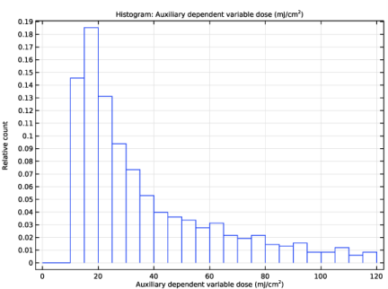
In the Settings window for Auxiliary Dependent Variable, type Absorbed Dose in the Label text field.
|
|
3
|
|
4
|
|
5
|
|
6
|
In the Dependent variable quantity table, enter the following settings:
|
|
1
|
|
2
|
|
1
|
|
2
|
|
3
|
|
4
|
|
1
|
|
2
|
|
3
|
|
4
|
|
5
|
|
6
|
|
1
|
|
2
|
|
1
|
|
2
|
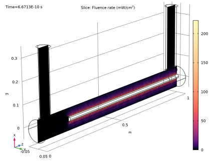
In the Settings window for Slice, click Replace Expression in the upper-right corner of the Expression section. From the menu, choose Component 1 (comp1)>Geometrical Optics>Heating and losses>gop.frc1.E0 - Fluence rate - W/m².
|
|
3
|
|
4
|
|
5
|
|
6
|
|
7
|
|
8
|
Click OK.
|
|
9
|
|
10
|
|
11
|
|
12
|
|
1
|
|
2
|
|
3
|
Find the Physics interfaces in study subsection. In the table, clear the Solve check boxes for Geometrical Optics (gop) and Particle Tracing for Fluid Flow (fpt).
|
|
4
|
|
5
|
|
6
|
|
1
|
|
2
|
Find the Values of variables not solved for subsection. From the Settings list, choose User controlled.
|
|
3
|
|
4
|
|
5
|
|
6
|
|
1
|
|
2
|
|
3
|
|
4
|
|
5
|
|
6
|
|
7
|
Click OK.
|
|
1
|
|
2
|
|
3
|
|
4
|
|
5
|
|
6
|
|
7
|
|
1
|
|
2
|
|
3
|
Find the Physics interfaces in study subsection. In the table, clear the Solve check boxes for Geometrical Optics (gop) and Turbulent Flow, k-ε (spf).
|
|
4
|
|
5
|
|
6
|
|
1
|
|
2
|
|
3
|
Click to expand the Values of Dependent Variables section. Find the Values of variables not solved for subsection. From the Settings list, choose User controlled.
|
|
4
|
|
5
|
|
6
|
|
1
|
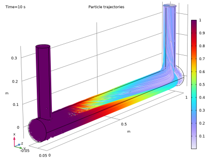
In the Model Builder window, expand the Results>Particle Trajectories (fpt)>Particle Trajectories 1 node, then click Color Expression 1.
|
|
2
|
|
3
|
|
4
|
|
5
|
|
6
|
Click OK.
|
|
1
|
|
2
|
|
3
|
|
1
|
|
2
|
|
3
|
|
4
|
|
1
|
|
2
|
|
3
|
|
4
|
|
5
|
|
6
|
|
7
|
|
8
|
|
1
|
|
2
|
In the Settings window for Filter, click Replace Expression in the upper-right corner of the Point Selection section. From the menu, choose Component 1 (comp1)>Particle Tracing for Fluid Flow>Particle Counter 1>fpt.pcnt1.rL - Logical expression for particle inclusion.
|