Slot-Die Coating with Channel Defect

Achieving uniform coating quality is important in several different industries: from optical coatings, semiconductor and electronics industry, through technologies utilizing thin membranes, to surface treatment of metals. Bad coating quality will compromise the performance of the products, or lead to complete failure in some cases.

Several different coating processes exist. This tutorial investigates the performance of a slot-die coating process, a so-called premetered coating method. In this process, the coating fluid is suspended from a thin slot die to a moving substrate. The final coating layer thickness is evaluated from the continuity relationship for a coating liquid. Therefore, the thickness of the liquid layer is determined by the slot gap, the coating fluid inlet velocity and the substrate speed.

The final goal of coating processes is to achieve a defect-free film of a desired thickness. However, manufacturing the uniform coating is not a trivial task, various flow instabilities or defects such as bubbles, ribbing, and rivulets are frequently observed in the process. The die geometry, the size of the slot and height above the substrate, together with the non-Newtonian fluid nature of the coating fluid are important to consider.

This tutorial demonstrates how to model the fluid flow in a polymer slot-die coating process using the interface and an inelastic non-Newtonian power law model for the polymer fluid.

Model Definition

Model Geometry

A typical setup of the slot-die coating process is shown in Figure 1.

Figure 1: Typical geometry for a slot-die coating process with the slot die positioned over a substrate.

This example models the coating process in 3D where the inlet channel is obstructed (Figure 2).

Figure 2: Model geometry.

More details about the model setup and COMSOL implementation can be found in the tutorial model 2D Non-Newtonian Slot-Die Coating.

Results

Figure 3 shows the evolution of the coating fluid interface for t = 0.05 s, t = 0.1 s, and t = 0.2 s.

Figure 3: Fluid interface at t = 0.03 s, t = 0.1 s, and t = 0.2 s.

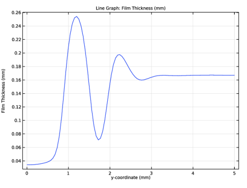
Figure 4 shows the variation of the film thickness across the outlet boundary. The channel defect leads to an uneven film thickness distribution. This can be partially mitigated by reducing the coating velocity.

Figure 4: Coating film thickness across the outlet boundary.

Reference

1. K.L. Bhamidipati, Detection and elimination of defects during manufacture of high-temperature polymer electrolyte membranes, PhD Thesis, Georgia Institute of Technology, 2011

Polymer_Flow_Module/Tutorials/slot_die_coating_3d

Modeling Instructions

From the menu, choose .

New

In the window, click

Model Wizard

In the window, click

In the tree, select .

Click .

Click

In the tree, select .

Click

Global Definitions

Parameters 1

In the window, under click .

In the window for , locate the section.

In the table, enter the following settings:


Name	Expression	Value	Description
W	0.2[mm]	2E-4 m	Inlet width
Hc	1.35[mm]	0.00135 m	Inlet height
W_dd	1.5[mm]	0.0015 m	Die width downstream
W_ud	1.35[mm]	0.00135 m	Die width upstream
alpha_u	45[deg]	0.7854 rad	Upstream die angle
alpha_d	55[deg]	0.95993 rad	Downstream die angle
L_u	5[mm]	0.005 m	Upstream length
L_d	10[mm]	0.01 m	Downstream length
H	0.2[mm]	2E-4 m	Channel height
Thickness	5[mm]	0.005 m	Thickness
U_wall	0.12[m/s]	0.12 m/s	Sliding wall velocity
U_in	0.1[m/s]	0.1 m/s	Inlet velocity
L_notch	1[mm]	0.001 m	Length of channel end notch

Geometry 1

In the window, expand the node, then click .

In the window for , locate the section.

From the list, choose .

Work Plane 1 (wp1)

In the toolbar, click

In the window, click .

In the window for , locate the section.

From the list, choose .

Click

Work Plane 1 (wp1)>Plane Geometry

In the window, click .

Work Plane 1 (wp1)>Rectangle 1 (r1)

In the toolbar, click

In the window for , locate the section.

In the text field, type W.

In the text field, type Hc.

Locate the section. In the text field, type -W/2.

In the text field, type H.

Click to expand the section. In the table, enter the following settings:


Layer name	Thickness (mm)
Layer 1	0.1

Work Plane 1 (wp1)>Polygon 1 (pol1)

In the toolbar, click

In the window for , locate the section.

In the table, enter the following settings:


xw (mm)	yw (mm)
-W/2	H
-W/2-W_ud	H
-W/2-W_ud-tan(alpha_u)*Hc	Hc+H
-W/2-L_u	Hc+H
-W/2-L_u	0
W/2+L_d	0
W/2+L_d	Hc+H
W/2+W_dd+tan(alpha_d)*Hc	Hc+H
W/2+W_dd	H

Extrude 1 (ext1)

In the window, right-click and choose .

In the window for , locate the section.

In the table, enter the following settings:


Distances (mm)
Thickness

Select the check box.

Click

Block 1 (blk1)

In the toolbar, click

In the window for , locate the section.

In the text field, type W.

In the text field, type L_notch.

In the text field, type Hc.

Locate the section. In the text field, type H.

In the text field, type -W/2.

Difference 1 (dif1)

In the toolbar, click

and choose .

Select the object only.

In the window for , locate the section.

Find the subsection. Click to select the

toggle button.

Select the object only.

Click

Global Definitions

Step 1 (step1)

In the toolbar, click

and choose .

In the window for , locate the section.

In the text field, type 0.01.

Click to expand the section. In the text field, type 0.02.

Materials

Air

In the window, under right-click and choose .

In the window for , type Air in the text field.

Locate the section. In the table, enter the following settings:


Property	Variable	Value	Unit	Property group
Density	rho	1.2	kg/m³	Basic
Dynamic viscosity	mu	1.8e-5	Pa·s	Basic

Coating Fluid

Right-click and choose .

In the window for , type Coating Fluid in the text field.

Go to the definition of the two phase model and select a non-newtonian power law model for the coating fluid. This will automatically enable the corresponding material parameters in the coating-fluid material.

Multiphysics

Two-Phase Flow, Phase Field 1 (tpf1)

In the window, under click .

In the window for , locate the section.

From the list, choose .

Locate the section. From the list, choose .

Find the subsection. From the list, choose .

Locate the section. From the list, choose . In the σ text field, type 0.049.

Click the

button in the toolbar.

In the dialog box, select in the tree.

In the tree, select the check box for the node .

Click .

In the window for , click to expand the section.

From the list, choose .

In the lρ text field, type 0.9.

From the list, choose .

In the lμ text field, type 0.9.

Select the check box.

To avoid spurious velocity and pressure oscillations due to the large density and viscosity ratios between the fluid, it can be advantageous to shift the surface tension force so that it is only applied in the heaviest phase. Note that this will reduce the computation time by several hours in this model.

Materials

Coating Fluid (mat2)

In the window, under click .

In the window for , locate the section.

In the table, enter the following settings:


Property	Variable	Value	Unit	Property group
Density	rho	1400	kg/m³	Basic
Fluid consistency coefficient	m_pow	7.77	Pa·s	Power law
Flow behavior index	n_pow	0.85	1	Power law