|
|
|
|
1
|
|
2
|
In the Select Physics tree, select Fluid Flow>Multiphase Flow>Two-Phase Flow, Phase Field>Laminar Flow.
|
|
3
|
Click Add.
|
|
4
|
Click
|
|
5
|
In the Select Study tree, select Preset Studies for Selected Multiphysics>Time Dependent with Phase Initialization.
|
|
6
|
Click
|
|
1
|
|
2
|
|
3
|
|
4
|
Browse to the model’s Application Libraries folder and double-click the file slot_die_coating_2d_parameters.txt.
|
|
1
|
|
2
|
|
3
|
|
4
|
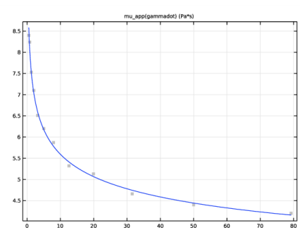
Browse to the model’s Application Libraries folder and double-click the file slot_die_coating_2d_viscosity_input.txt.
|
|
5
|
Locate the Column Settings section. In the table, click to select the cell at row number 1 and column number 1.
|
|
6
|
|
7
|
|
9
|
|
10
|
|
11
|
|
12
|
Locate the Parameters section. In the table, enter the following settings:
|
|
13
|
Click
|
|
14
|
|
1
|
|
2
|
|
3
|
|
4
|
|
1
|
|
2
|
|
3
|
|
4
|
|
1
|
|
2
|
|
3
|
|
4
|
|
5
|
|
6
|
|
7
|
Click to expand the Layers section. In the table, enter the following settings:
|
|
8
|
|
1
|
|
2
|
|
4
|
|
5
|
|
1
|
|
2
|
|
3
|
|
4
|
|
1
|
|
2
|
|
3
|
|
1
|
In the Model Builder window, under Component 1 (comp1)>Multiphysics click Two-Phase Flow, Phase Field 1 (tpf1).
|
|
2
|
|
3
|
|
1
|
In the Model Builder window, under Component 1 (comp1)>Materials>Multiphase Material 1 (mpmat1) click Phase 1 (mpmat1.phase1).
|
|
2
|
|
3
|
Click
|
|
1
|
|
2
|
In the tree, select Built-in>Air.
|
|
3
|
Click OK.
|
|
1
|
In the Model Builder window, under Component 1 (comp1)>Materials>Multiphase Material 1 (mpmat1) click Phase 2 (mpmat1.phase2).
|
|
2
|
|
3
|
|
1
|
|
2
|
|
3
|
Locate the Material Properties section. In the Material properties tree, select Fluid Flow>Inelastic Non-Newtonian>Power Law.
|
|
4
|
|
5
|
|
1
|
In the Model Builder window, under Component 1 (comp1)>Materials click Multiphase Material 1 (mpmat1).
|
|
2
|
|
4
|
|
5
|
|
6
|
|
7
|
|
8
|
|
9
|
|
10
|
Click OK.
|
|
1
|
In the Model Builder window, under Component 1 (comp1) right-click Laminar Flow (spf) and choose Wall.
|
|
3
|
|
4
|
|
5
|
|
6
|
|
1
|
|
3
|
|
4
|
|
5
|
|
1
|
|
1
|
In the Model Builder window, under Component 1 (comp1)>Phase Field (pf) click Initial Values, Fluid 2.
|
|
1
|
|
2
|
|
3
|
|
1
|
|
2
|
|
3
|
|
1
|
|
1
|
|
3
|
|
4
|
|
1
|
|
2
|
|
3
|
|
4
|
Click OK.
|
|
5
|
In the Model Builder window, under Component 1 (comp1)>Multiphysics click Two-Phase Flow, Phase Field 1 (tpf1).
|
|
6
|
In the Settings window for Two-Phase Flow, Phase Field, click to expand the Advanced Settings section.
|
|
7
|
|
8
|
Locate the Surface Tension section. From the Surface tension coefficient list, choose User defined. In the σ text field, type 0.049.
|
|
1
|
|
2
|
|
3
|
Select the Plot check box.
|
|
4
|
|
5
|
|
6
|
|
7
|
|
1
|
|
2
|
|
3
|
|
4
|
|
5
|
|
6
|
|
7
|
|
8
|
|
1
|
|
2
|
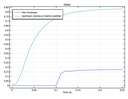
In the Settings window for 1D Plot Group, type Film Thickness and Upstream Meniscus Position in the Label text field.
|
|
3
|
|
1
|
|
2
|
|
4
|