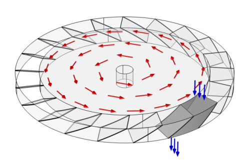
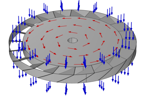
PDF

Turbomolecular Pump
Introduction
Turbomolecular pumps (TMPs) are widely used in vacuum system design. A TMP is a bladed molecular turbine that compresses gases by momentum transfer from the rapidly rotating blades of the rotor to the gas molecules. In the free molecular flow range (typically less than 10-1 Pa), the particles collide primarily with the rotor, rather than each other, resulting in an efficient pumping process. The following assumptions are made:
This 3D model uses the Mathematical Particle Tracing interface to evaluate the performance of a simple turbomolecular pump in the free molecular flow regime. While the Free Molecular Flow interface provides an efficient and deterministic calculation of gas density in the free molecular flow regime, it uses the angular coefficient method which is only applicable for molecules that are moving much faster than any object in the geometry. For TMPs, where the blades move over similar time scales as the molecules themselves, this requirement is not satisfied, so a Monte Carlo approach is used instead.
The particle trajectories are computed in a rotating frame of reference, attached to the rotor, in which the fictitious centrifugal and Coriolis forces are automatically taken into account. The model shows the effect of the blade velocity ratio on the pumping characteristics, including the transmission probability, maximum compression ratio, and maximum speed factor.
Model Definition
A TMP may include a large number of stages, or rows of blades. For the TMP design considered in this example, each row of blades is arranged in a ring, and each blade is held at an angle. By rotating these rings of blades, a change in gas density in the axial direction is produced because the inclined blades are more likely to permit a gas molecule to cross the stage in one direction than in the opposite direction. The stage is called a rotor if it is allowed to rotate, or a stator if it is held in a fixed position. A single-stage rotor is illustrated in Figure 1; if the blades rotate counterclockwise as indicated by the red arrows, molecules are more likely to cross the stage going downward (as indicated by the blue arrows) than they are to go upward. Due to sector symmetry, the geometry can be simplified by considering only the gap between two blades, such as the region highlighted in Figure 2.
Figure 1: Full geometry of a turbomolecular pump stage.
Figure 2: Geometry of a turbomolecular pump stage, where a single unit cell and the molecules entering and leaving it have been highlighted.
As in Ref. 1, the pump stage consists of 36 blades, each inclined at a 30 degree angle. The ratio of the root radius to the tip radius is 0.8. Note that if the root-to-tip ratio is very close to unity, the centrifugal and Coriolis forces can be neglected to some extent, allowing a less computationally intensive quasi-2D model to be used instead.
The relevant pump characteristics are based on the transmission probability of argon atoms from the inlet to the outlet M12 and the transmission probability from the outlet back to the inlet M21 (both dimensionless). In order to compute these transmission probabilities, the model uses two Inlet features to release particles on either side of the pump and two Outlet features to capture particles that reach the boundaries. The Particle Counter can be used to compute the number of particles from each Inlet that reach each Outlet.
Each Inlet releases argon atoms with a Lambertian distribution of initial directions and a Maxwellian distribution of initial speeds. The most probable speed of particles in the Maxwellian distribution vp (SI unit: m/s) is
where
kB = 1.380649 × 10-23 J/K is the Boltzmann constant,
T = 300 K is the ambient temperature,
M = 39.948 g/mol is the molar mass of argon, and
NA = 6.02214076 × 1023 1/mol is the Avogadro constant.
This gives a most probable speed of approximately vp = 353 m/s.
The root wall, tip wall, and blade surfaces use the dedicated Thermal Re-Emission boundary condition, in which incident molecules are adsorbed onto the wall and then immediately released back into the modeling domain with a random velocity based on the surface temperature. The root wall and blades are stationary with respect to the rotating frame of reference, while the tip wall is stationary with respect to the inertial (laboratory) frame, and therefore moves relative to the rotating frame.
Modern turbomolecular pumps can operate at very high rotor speeds reaching 90,000 revolutions per minute. In this model, the angular velocity of the pump is specified in terms of the dimensionless blade velocity ratio C, defined as
(1)
where vb (SI unit: m/s) is the blade velocity, or the rms velocity magnitude of the rotating frame. The transmission probability is computed for different values of C from 0 to 4 using a Parametric Sweep; the maximum value C = 4 corresponds to a blade velocity of approximately vb = 1415 m/s.
About Particle Tracing in Rotating Domains
To model the motion of the argon atoms in a rotating frame, a set of second-order differential equations for the components of the particle position q (SI unit: m) are solved:
where
Fcen is the centrifugal force,
Fcor is the Coriolis force,
Feul is the Euler force,
Ω (SI unit: rad/s) is the angular velocity of the rotating frame, and
r (SI unit: m) is the displacement from the center of rotation to the atom’s position.
All of these fictitious forces are automatically defined by the Rotating Frame feature. In this example, the frame rotates at constant angular velocity, so the Euler force is zero.
Results and Discussion
The Parametric Sweep over the velocity ratio C begins at C = 0 and ends at C = 4 with intervals of 0.5. The final particle positions for six of these values are shown in Figure 3. The green particles begin at the top boundary while the red particles are released at the bottom boundary. As the velocity ratio increases, more green particles are able to cross from the top to the bottom, but fewer red particles can cross from the bottom to the top. Both effects cause the compression ratio of the turbopump stage to increase.
Figure 3: Final particle positions for different values of the blade velocity ratio C.
The transmission probabilities M12 and M21 for propagation in the forward and reverse directions are shown in Figure 4 and Figure 5, respectively. As expected, the transmission probabilities are almost equal when the blades are at rest (C = 0) because there is no distinction between the forward and reverse directions. As the blades begin to rotate faster, particles are more likely to be transmitted in the forward direction due to the momentum transferred to the argon atoms from the rotating walls.
Figure 4: Fraction of particles transmitted from the inlet to the outlet M12, as a function of the blade velocity ratio C.
Figure 5: Fraction of particles transmitted from the outlet to the inlet M21, as a function of the blade velocity ratio C.
Multiple-bladed structures with several disks provide adequate compression and speed to make a functional pump. The blades nearest the inlet are usually designed to have a high pumping speed and a low compression ratio. The blades nearest the outlet are designed to have a high compression ratio and a low pumping speed.
The maximum compression ratio Kmax is defined by
(2)
and the maximum speed factor Wmax by
(3)
Figure 6 and Figure 7 show the variation of these values as the blade velocity is increased. Compare these results to the corresponding plots in Ref. 1. The compression ratio is expected to increase monotonically. If C is further increased, some statistical noise is expected as the denominator M21 becomes very small. In such cases, consider increasing the number of model particles for a more statistically converged solution.
Figure 6: Maximum compression ratio Kmax, as a function of the blade velocity ratio C.
Figure 7: Maximum speed factor Wmax, as a function of the blade velocity ratio C.
Reference
1. Y. Li and others, “Numerical investigation of three turbomolecular pump models in the free molecular flow range,” Vacuum, vol. 101, pp. 337–344, 2014.
Application Library path: Particle_Tracing_Module/Vacuum_Systems/turbomolecular_pump
Modeling Instructions
From the File menu, choose New.
New
In the New window, click  Model Wizard.
Model Wizard
1
In the Model Wizard window, click  3D.
2
In the Select Physics tree, select Mathematics>Mathematical Particle Tracing (pt).
3
Click Add.
4
Click  Study.
5
In the Select Study tree, select General Studies>Time Dependent.
6
Root
Insert the prepared geometry sequence from file. You can read the instructions for creating the geometry in the appendix.
Geometry 1
1
In the Geometry toolbar, click Insert Sequence and choose Insert Sequence.
2
3
In the Geometry toolbar, click  Build All.
4
Click the  Zoom Extents button in the Graphics toolbar.
Component 1 (comp1)
1
In the Model Builder window, click Component 1 (comp1).
2
In the Settings window for Component, locate the Curved Mesh Elements section.
3
From the Geometry shape function list, choose Linear Lagrange. Linear geometry shape order is the most robust option for modeling diffuse scattering at convex curved surfaces, such as the tip wall in this geometry.
Global Definitions
Geometry Parameters
1
In the Model Builder window, under Global Definitions click Parameters 1.
2
In the Settings window for Parameters, type Geometry Parameters in the Label text field.
Physics Parameters
1
In the Home toolbar, click  Parameters and choose Add>Parameters.
2
In the Settings window for Parameters, type Physics Parameters in the Label text field.
3
Locate the Parameters section. Click  Load from File.
4
Definitions
Variables 1
1
In the Model Builder window, under Component 1 (comp1) right-click Definitions and choose Variables.
2
In the Settings window for Variables, locate the Variables section.
3
Mathematical Particle Tracing (pt)
1
In the Model Builder window, under Component 1 (comp1) click Mathematical Particle Tracing (pt).
2
In the Settings window for Mathematical Particle Tracing, locate the Particle Release and Propagation section.
3
In the Maximum number of secondary particles text field, type 0.
Particle Properties 1
1
In the Model Builder window, under Component 1 (comp1)>Mathematical Particle Tracing (pt) click Particle Properties 1.
2
In the Settings window for Particle Properties, locate the Particle Mass section.
3
In the mp text field, type m.
Rotating Frame 1
1
In the Physics toolbar, click  Domains and choose Rotating Frame.
2
In the Settings window for Rotating Frame, locate the Rotating Frame section.
3
In the Ω text field, type omega.
Inlet 1
1
In the Physics toolbar, click  Boundaries and choose Inlet.
2
In the Settings window for Inlet, locate the Boundary Selection section.
3
From the Selection list, choose Inlet Boundary.
4
Locate the Initial Position section. From the Initial position list, choose Density.
5
In the N text field, type 10000.
6
Locate the Initial Velocity section. From the Initial velocity list, choose Thermal.
7
In the T text field, type T0.
8
Click to expand the Advanced Settings section. Select the Subtract moving frame velocity from initial particle velocity check box.
Inlet 2
1
In the Physics toolbar, click  Boundaries and choose Inlet.
2
In the Settings window for Inlet, locate the Boundary Selection section.
3
From the Selection list, choose Outlet Boundary.
4
Locate the Initial Position section. From the Initial position list, choose Density.
5
In the N text field, type 10000.
6
Locate the Initial Velocity section. From the Initial velocity list, choose Thermal.
7
In the T text field, type T0.
8
Locate the Advanced Settings section. Select the Subtract moving frame velocity from initial particle velocity check box.
Particle Counter (Inlet 1 Transmission)
1
In the Physics toolbar, click  Boundaries and choose Particle Counter.
2
In the Settings window for Particle Counter, type Particle Counter (Inlet 1 Transmission) in the Label text field.
3
Locate the Boundary Selection section. From the Selection list, choose Outlet Boundary.
4
Locate the Particle Counter section. From the Release feature list, choose Inlet 1.
Particle Counter (Inlet 2 Transmission)
1
In the Physics toolbar, click  Boundaries and choose Particle Counter.
2
In the Settings window for Particle Counter, type Particle Counter (Inlet 2 Transmission) in the Label text field.
3
Locate the Boundary Selection section. From the Selection list, choose Inlet Boundary.
4
Locate the Particle Counter section. From the Release feature list, choose Inlet 2.
Root and Blade Surfaces
1
In the Physics toolbar, click  Boundaries and choose Thermal Re-Emission.
2
In the Settings window for Thermal Re-Emission, type Root and Blade Surfaces in the Label text field.
3
Locate the Boundary Selection section. From the Selection list, choose All Moving Walls.
4
Locate the Wall Properties section. In the T text field, type T0.
Tip Wall
1
In the Physics toolbar, click  Boundaries and choose Thermal Re-Emission.
2
In the Settings window for Thermal Re-Emission, type Tip Wall in the Label text field.
3
Locate the Boundary Selection section. From the Selection list, choose Tip Wall.
4
Locate the Wall Properties section. In the T text field, type T0.
5
Locate the Frame Settings section. Select the Subtract moving frame velocity from reflected particle velocity check box.
Mesh 1
1
In the Model Builder window, under Component 1 (comp1) click Mesh 1.
2
In the Settings window for Mesh, locate the Physics-Controlled Mesh section.
3
From the Element size list, choose Extra fine.
4
Click  Build All.
Study 1
Parametric Sweep
1
In the Study toolbar, click  Parametric Sweep.
2
In the Settings window for Parametric Sweep, locate the Study Settings section.
3
4
Step 1: Time Dependent
1
In the Model Builder window, click Step 1: Time Dependent.
2
In the Settings window for Time Dependent, locate the Study Settings section.
3
From the Time unit list, choose ms.
4
In the Output times text field, type range(0,0.01,0.5).
5
In the Study toolbar, click  Compute.
Results
Particle Trajectories (pt)
The default plot shows the particle positions at the final time step for the highest value of the speed factor. The particles are colored by velocity. Instead, color them by release feature to better visualize the transmission probability across the stage.
1
In the Model Builder window, expand the Particle Trajectories (pt) node.
Color Expression 1
1
In the Model Builder window, expand the Results>Particle Trajectories (pt)>Particle Trajectories 1 node, then click Color Expression 1.
2
In the Settings window for Color Expression, click Replace Expression in the upper-right corner of the Expression section. From the menu, choose Component 1 (comp1)>Mathematical Particle Tracing>Particle statistics>pt.prf - Particle release feature.
3
Locate the Coloring and Style section. Click  Change Color Table.
4
In the Color Table dialog box, select Traffic>TrafficLight in the tree.
5
Particle Trajectories (pt)
1
In the Model Builder window, under Results click Particle Trajectories (pt).
2
In the Settings window for 3D Plot Group, locate the Color Legend section.
3
Clear the Show legends check box.
4
In the Particle Trajectories (pt) toolbar, click  Plot.
5
Click the  Zoom Extents button in the Graphics toolbar.
The green particles were released from the top boundary while the red particles were released from the bottom boundary. Plot the particle trajectories at different values of the dimensionless speed factor, C, to observe how the rotating frame breaks the symmetry of the red and green particles. Several plots are shown in Figure 3.
M12
1
In the Home toolbar, click  Add Plot Group and choose 1D Plot Group.
2
In the Settings window for 1D Plot Group, type M12 in the Label text field.
3
Locate the Data section. From the Dataset list, choose Study 1/Parametric Solutions 1 (sol2).
4
From the Time selection list, choose Last.
5
Locate the Legend section. Clear the Show legends check box.
Global 1
1
Right-click M12 and choose Global.
2
In the Settings window for Global, locate the y-Axis Data section.
3
4
Locate the x-Axis Data section. From the Axis source data list, choose C.
5
Click to expand the Coloring and Style section. From the Color list, choose Black.
6
Find the Line markers subsection. From the Marker list, choose Circle.
7
In the M12 toolbar, click  Plot. Compare the resulting plot with Figure 4.
M21
1
In the Model Builder window, right-click M12 and choose Duplicate.
2
In the Settings window for 1D Plot Group, type M21 in the Label text field.
Global 1
1
In the Model Builder window, expand the M21 node, then click Global 1.
2
In the Settings window for Global, locate the y-Axis Data section.
3
4
In the M21 toolbar, click  Plot. Compare the resulting plot with Figure 5.
Kmax
1
In the Model Builder window, right-click M21 and choose Duplicate.
2
In the Settings window for 1D Plot Group, type Kmax in the Label text field.
Global 1
1
In the Model Builder window, expand the Kmax node, then click Global 1.
2
In the Settings window for Global, locate the y-Axis Data section.
3
4
In the Kmax toolbar, click  Plot.
5
Click the  y-Axis Log Scale button in the Graphics toolbar. Compare the resulting plot with Figure 6.
Wmax
1
In the Model Builder window, right-click Kmax and choose Duplicate.
2
In the Settings window for 1D Plot Group, type Wmax in the Label text field.
Global 1
1
In the Model Builder window, expand the Wmax node, then click Global 1.
2
In the Settings window for Global, locate the y-Axis Data section.
3
4
In the Wmax toolbar, click  Plot.
5
Click the  y-Axis Log Scale button in the Graphics toolbar. Compare the resulting plot with Figure 7.
 
Appendix — Geometry Instructions
From the File menu, choose New.
New
In the New window, click  Blank Model.
Add Component
In the Home toolbar, click  Add Component and choose 3D.
Global Definitions
Parameters 1
1
In the Model Builder window, under Global Definitions click Parameters 1.
2
In the Settings window for Parameters, locate the Parameters section.
3
Click  Load from File.
4
Geometry 1
Cylinder 1 (cyl1)
1
In the Geometry toolbar, click  Cylinder.
2
In the Settings window for Cylinder, locate the Size and Shape section.
3
In the Radius text field, type rtip.
4
In the Height text field, type rh.
5
Locate the Position section. In the z text field, type -rh/2.
6
Locate the Rotation Angle section. In the Rotation text field, type 30.
Cylinder 2 (cyl2)
1
Right-click Cylinder 1 (cyl1) and choose Duplicate.
2
In the Settings window for Cylinder, locate the Size and Shape section.
3
In the Radius text field, type rroot.
Difference 1 (dif1)
1
In the Geometry toolbar, click  Booleans and Partitions and choose Difference.
2
3
In the Settings window for Difference, locate the Difference section.
4
Find the Objects to subtract subsection. Click to select the  Activate Selection toggle button.
5
6
Click  Build Selected.
Work Plane 1 (wp1)
1
In the Geometry toolbar, click  Work Plane.
2
In the Settings window for Work Plane, locate the Plane Definition section.
3
From the Plane type list, choose Coordinates.
4
In row Point 1, set x to wp11x.
5
In row Point 1, set y to wp11y.
6
In row Point 1, set z to wp11z.
7
In row Point 2, set x to wp12x.
8
In row Point 2, set y to wp12y.
9
In row Point 2, set z to wp12z.
10
In row Point 3, set x to wp13x.
11
In row Point 3, set y to wp13y.
12
In row Point 3, set z to wp13z.
Work Plane 2 (wp2)
1
In the Geometry toolbar, click  Work Plane.
2
In the Settings window for Work Plane, locate the Plane Definition section.
3
From the Plane type list, choose Coordinates.
4
In row Point 1, set x to wp21x.
5
In row Point 1, set y to wp21y.
6
In row Point 1, set z to wp21z.
7
In row Point 2, set x to wp22x.
8
In row Point 2, set y to wp22y.
9
In row Point 2, set z to wp22z.
10
In row Point 3, set x to wp23x.
11
In row Point 3, set y to wp23y.
12
In row Point 3, set z to wp23z.
Partition Objects 1 (par1)
1
In the Geometry toolbar, click  Booleans and Partitions and choose Partition Objects.
2
3
In the Settings window for Partition Objects, locate the Partition Objects section.
4
From the Partition with list, choose Work plane.
5
From the Work plane list, choose Work Plane 1 (wp1).
Partition Objects 2 (par2)
1
In the Geometry toolbar, click  Booleans and Partitions and choose Partition Objects.
2
3
In the Settings window for Partition Objects, locate the Partition Objects section.
4
From the Partition with list, choose Work plane.
Delete Entities 1 (del1)
1
In the Model Builder window, right-click Geometry 1 and choose Delete Entities.
2
On the object par2, select Boundary 7 only.
3
In the Settings window for Delete Entities, locate the Entities or Objects to Delete section.
4
From the Geometric entity level list, choose Domain.
5
On the object par2, select Domains 1–3 only.
6
Click  Build All Objects.
7
Click the  Zoom Extents button in the Graphics toolbar.
Inlet Boundary
1
In the Geometry toolbar, click  Selections and choose Explicit Selection.
2
In the Settings window for Explicit Selection, type Inlet Boundary in the Label text field.
3
Locate the Entities to Select section. From the Geometric entity level list, choose Boundary.
4
On the object del1, select Boundary 3 only.
Outlet Boundary
1
In the Geometry toolbar, click  Selections and choose Explicit Selection.
2
In the Settings window for Explicit Selection, type Outlet Boundary in the Label text field.
3
Locate the Entities to Select section. From the Geometric entity level list, choose Boundary.
4
On the object del1, select Boundary 4 only.
Root Wall
1
In the Geometry toolbar, click  Selections and choose Explicit Selection.
2
In the Settings window for Explicit Selection, type Root Wall in the Label text field.
3
Locate the Entities to Select section. From the Geometric entity level list, choose Boundary.
4
On the object del1, select Boundary 1 only.
Tip Wall
1
In the Geometry toolbar, click  Selections and choose Explicit Selection.
2
In the Settings window for Explicit Selection, type Tip Wall in the Label text field.
3
Locate the Entities to Select section. From the Geometric entity level list, choose Boundary.
4
On the object del1, select Boundary 6 only.
Blade Surfaces
1
In the Geometry toolbar, click  Selections and choose Explicit Selection.
2
In the Settings window for Explicit Selection, type Blade Surfaces in the Label text field.
3
Locate the Entities to Select section. From the Geometric entity level list, choose Boundary.
4
On the object del1, select Boundaries 2 and 5 only.
All Moving Walls
1
In the Geometry toolbar, click  Selections and choose Union Selection.
2
In the Settings window for Union Selection, type All Moving Walls in the Label text field.
3
Locate the Geometric Entity Level section. From the Level list, choose Boundary.
4
Locate the Input Entities section. Click  Add.
5
In the Add dialog box, in the Selections to add list, choose Root Wall and Blade Surfaces.
6