PDF

Relativistic Diverging Electron Beam
Introduction
When modeling the propagation of charged particle beams at high currents and relativistic speeds, the space charge and beam current create significant electric and magnetic forces that tend to expand and focus the beam, respectively. The Charged Particle Tracing interface can use an iterative procedure to efficiently compute the strongly coupled particle trajectories and electric and magnetic fields for a beam operating at constant current. To validate the model, the change in beam radius from the waist position is compared to an analytic expression for the shape of a relativistic beam envelope.
Note: This application requires the AC/DC Module and Particle Tracing Module.
Model Definition
This model is almost identical to the Electron Beam Divergence Due to Self Potential model but with higher beam current and particle velocities. To accurately compute the relativistic particle trajectories, a correction has to be applied to the mass of the electrons,
(1)
where
mr = 9.10938356 × 10-31 kg is the rest mass of the electron,
c = 2.99792458 × 108 m/s is the speed of light in a vacuum, and
v (SI unit: m/s) is the magnitude of the electron velocity.
At relativistic speeds, the electron beam generates a magnetic field that exerts a significant magnetic force on the electrons. The ratio of self-induced magnetic and electric forces is proportional to β2 = (v/c)2 (Ref. 1).
As in the nonrelativistic case, the shape of the beam envelope has the analytic solution
(2)
where z (SI unit: m) is the distance from the beam waist, R0 (SI unit: m) is the waist radius, K (dimensionless) is the generalized beam perveance,
γ (dimensionless) is the relativistic factor defined as
(3)
χ (dimensionless) is the ratio of the beam radius to the beam waist radius, and
(4)
This analytical expression for the relationship between axial position and beam envelope radius is used to determine the accuracy of the solution.
Results and Discussion
The electron trajectories are plotted in Figure 1 while the electric potential distribution and magnetic flux norm are respectively shown on Figure 2, and Figure 3. The distance from the beam waist as a function of beam radius is compared to the result of Equation 2 using a Global Evaluation. The results agree to within a few percentage points. The sources of numerical error include discretization error of the charge density and current density, both of which use constant shape functions within each mesh element.
Figure 1: A beam of electrons with a waist located at z = 0 diverges due to transverse beam forces. The color represents the radial displacement of each electron from its initial position.
Figure 2: Electric potential in the relativistic beam. The magnitude of the potential is greatest at the beam waist.
Figure 3: Magnetic flux density norm in the beam.
Reference
1. S. Humphries, Charged Particle Beams, Dover Publications, New York, 2013.
Application Library path: Particle_Tracing_Module/Charged_Particle_Tracing/electron_beam_divergence_relativistic
Model Instructions
From the File menu, choose New.
New
In the New window, click  Model Wizard.
Model Wizard
1
In the Model Wizard window, click  3D.
2
In the Select Physics tree, select AC/DC>Particle Tracing>Particle Field Interaction, Relativistic.
3
Click Add.
4
Click  Study.
5
In the Select Study tree, select Preset Studies for Selected Physics Interfaces>Charged Particle Tracing>Bidirectionally Coupled Particle Tracing.
6
Global Definitions
To save time, the parameters can be loaded from a file.
Parameters 1
1
In the Model Builder window, under Global Definitions click Parameters 1.
2
In the Settings window for Parameters, locate the Parameters section.
3
Click  Load from File.
4
Browse to the model’s Application Libraries folder and double-click the file electron_beam_divergence_relativistic_parameters.txt.
Geometry 1
Cylinder 1 (cyl1)
1
In the Geometry toolbar, click  Cylinder.
2
In the Settings window for Cylinder, locate the Size and Shape section.
3
In the Radius text field, type r0.
4
In the Height text field, type L.
5
Click  Build Selected.
Work Plane 1 (wp1)
1
In the Geometry toolbar, click  Work Plane.
2
In the Settings window for Work Plane, locate the Plane Definition section.
3
From the Plane type list, choose Face parallel.
4
On the object cyl1, select Boundary 3 only.
It might be easier to select the correct boundary by using the Selection List window. To open this window, in the Home toolbar click Windows and choose Selection List. (If you are running the cross-platform desktop, you find Windows in the main menu.)
5
Click  Show Work Plane.
Work Plane 1 (wp1)>Circle 1 (c1)
1
In the Work Plane toolbar, click  Circle.
2
In the Settings window for Circle, locate the Size and Shape section.
3
In the Radius text field, type r0beam.
4
Click  Build Selected.
Add Material
1
In the Home toolbar, click  Add Material to open the Add Material window.
2
Go to the Add Material window.
3
In the tree, select Built-in>Perfect vacuum.
4
Click Add to Component in the window toolbar.
5
In the Home toolbar, click  Add Material to close the Add Material window.
Definitions
Variables 1
1
In the Home toolbar, click  Variables and choose Local Variables.
2
In the Settings window for Variables, locate the Variables section.
3
Electrostatics (es)
Ground 1
1
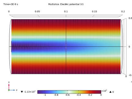
In the Model Builder window, under Component 1 (comp1) right-click Electrostatics (es) and choose Ground.
2
Charged Particle Tracing (cpt)
Particle Properties 1
1
In the Model Builder window, under Component 1 (comp1)>Charged Particle Tracing (cpt) click Particle Properties 1.
2
In the Settings window for Particle Properties, locate the Particle Species section.
3
From the Particle species list, choose Electron.
Inlet 1
1
In the Physics toolbar, click  Boundaries and choose Inlet.
2
3
In the Settings window for Inlet, locate the Release Current Magnitude section.
4
In the I text field, type Ibeam.
5
Locate the Initial Position section. From the Initial position list, choose Density.
6
In the N text field, type 1000.
7
Locate the Initial Velocity section. Specify the v0 vector as
Electric Force 1
1
In the Model Builder window, click Electric Force 1.
2
In the Settings window for Electric Force, locate the Electric Force section.
3
From the E list, choose Electric field (es/ccn1).
4
Locate the Advanced Settings section. Select the Use piecewise polynomial recovery on field check box.
Magnetic Force 1
1
In the Model Builder window, click Magnetic Force 1.
2
In the Settings window for Magnetic Force, locate the Magnetic Force section.
3
From the B list, choose Magnetic flux density (mf/al1).
4
Locate the Advanced Settings section. Select the Use piecewise polynomial recovery on field check box.
Mesh 1
1
In the Model Builder window, under Component 1 (comp1) click Mesh 1.
2
In the Settings window for Mesh, locate the Sequence Type section.
3
From the list, choose User-controlled mesh.
Size
1
In the Model Builder window, under Component 1 (comp1)>Mesh 1 click Size.
2
In the Settings window for Size, click to expand the Element Size Parameters section.
3
In the Maximum element size text field, type hmax.
4
Click  Build All.
Study 1
Step 1: Bidirectionally Coupled Particle Tracing
1
In the Model Builder window, under Study 1 click Step 1: Bidirectionally Coupled Particle Tracing.
2
In the Settings window for Bidirectionally Coupled Particle Tracing, locate the Study Settings section.
3
In the Output times text field, type range(0,1.0e-10,3e-9).
4
From the Tolerance list, choose User controlled.
5
In the Relative tolerance text field, type 1.0E-5.
6
Locate the Iterations section. From the Termination method list, choose Convergence of global variable.
7
In the Global variable text field, type qrmax.
8
In the Relative tolerance text field, type 1E-5.
9
In the Relative tolerance threshold text field, type 0.015.
10
In the Maximum number of iterations text field, type 8.
Solution 1 (sol1)
1
In the Study toolbar, click  Show Default Solver.
2
In the Model Builder window, expand the Solution 1 (sol1) node, then click Compile Equations: Bidirectionally Coupled Particle Tracing (2).
3
In the Settings window for Compile Equations, locate the Study and Step section.
4
Select the Split complex variables in real and imaginary parts check box.
5
In the Study toolbar, click  Compute.
Results
Plot the trajectories of the electrons, using a Color Expression to observe their radial displacement over time.
Particle Trajectories 1
1
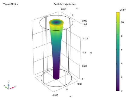
In the Model Builder window, expand the Results>Particle Trajectories (cpt) node, then click Particle Trajectories 1.
2
In the Settings window for Particle Trajectories, locate the Coloring and Style section.
3
Find the Line style subsection. From the Type list, choose Line.
Color Expression 1
1
In the Model Builder window, expand the Particle Trajectories 1 node, then click Color Expression 1.
2
In the Settings window for Color Expression, locate the Expression section.
3
In the Expression text field, type qr-at(0,qr).
4
Locate the Coloring and Style section. Click  Change Color Table.
5
In the Color Table dialog box, select Linear>Viridis in the tree.
6
7
In the Particle Trajectories (cpt) toolbar, click  Plot.
8
Click the  Zoom Extents button in the Graphics toolbar. This plot should look like Figure 1.
Electric Potential (es)
1
In the Model Builder window, under Results click Electric Potential (es).
2
In the Settings window for 3D Plot Group, locate the Color Legend section.
3
From the Position list, choose Bottom.
4
In the Graphics window toolbar, clicknext to  Go to Default View, then choose Go to ZX View. This plot should look like Figure 2.
Magnetic Flux Density Norm (mf)
1
In the Model Builder window, click Magnetic Flux Density Norm (mf).
2
In the Settings window for 3D Plot Group, locate the Color Legend section.
3
From the Position list, choose Bottom. This plot should look like Figure 3.
Global Evaluation 1
1
In the Results toolbar, click  Global Evaluation.
2
In the Settings window for Global Evaluation, locate the Data section.
3
From the Time selection list, choose Last.
4
Locate the Expressions section. In the table, enter the following settings:
5
Click  Evaluate.