Electron Beam Divergence Due to Self Potential

When modeling the propagation of a charged particle beam at a high current, the electric field due to the space charge of the beam significantly affects the trajectories of the charged particles. Perturbations to these trajectories, in turn, affect the space charge distribution. In order to accurately predict the properties of the beam, the particle trajectories and fields must be computed in a self-consistent manner. The Charged Particle Tracing interface can use an iterative procedure to efficiently compute the strongly coupled particle trajectories and electric field for systems operating under steady-state conditions. Such a procedure reduces the required number of model particles by several orders of magnitude, compared to methods based on explicit modeling of Coulomb interactions between the beam particles. To validate the model, the change in beam radius from the waist position is compared to an analytic expression for the shape a nonrelativistic, paraxial beam envelope.

Model Definition

This model computes the shape of an electron beam propagating through free space. When the magnitude of the beam current is large enough that Coulomb interactions are significant, the shape of the beam may be determined by solving a set of strongly coupled equations for the beam potential and the electron trajectories,

where

•

me = 9.10938356 × 10-31 kg is the electron mass,

•

e = 1.602176634 × 10-19 C is the elementary charge,

•

ε0 = 8.854187817 × 10-12 F/m is the permittivity of vacuum,

•

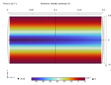
V (SI unit: V) is the electric potential,

•

N (dimensionless) is the total number of particles,

•

r (SI unit: m) is the position vector,

•

qi (SI unit: m) is the position of the ith particle, and

•

δ (SI unit: 1/m3) is the Dirac delta function.

The beam electrons are assumed nonrelativistic so that magnetic forces can be neglected. Modeling the beam electrons and the resulting electric potential using a time-dependent study would require a very large number of model particles to be released at a large number of time intervals. Instead, this model computes the shape of the electron beam by coupling a analysis of the particle trajectories to a analysis of the electric potential. The two different types of solver are combined using the dedicated study step. This algorithm is suitable for modeling beams which operate at steady-state conditions. It consists of the following steps:

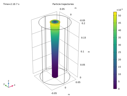
Compute the particle trajectories in the time domain, ignoring Coulomb forces. Compute the space charge density using the node.

Compute the stationary electric potential due to the space charge density of the beam.

Use the electric potential calculated in step 2 to compute the perturbed particle trajectories. Recalculate the space charge density using these perturbed trajectories.

Repeat steps 2 and 3 until a specified number of iterations has been reached, or until some other user-specified convergence criterion has been met.

After several iterations, the particle trajectories and the corresponding space charge density and electric field reach a stable, self-consistent solution. For a nonrelativistic, paraxial beam of electrons, the shape of the beam envelope is given by Ref. 1 should follow the equation

(1)

where z (SI unit: m) is the distance from the beam waist, R0 (SI unit: m) is the waist radius, K (dimensionless) is the generalized beam perveance,

χ (dimensionless) is the ratio of the beam radius to the beam waist radius, and

(2)

In this example, each model particle actually represents a continuous stream of electrons, released at regular time intervals, rather than the instantaneous position of a single charge. For the purpose of modeling particle-field interactions, each model particle leaves behind a trail of space charge in its wake. The contribution of each particle to the total space charge density of the beam is found by evaluating the sum

where frel (SI unit: 1/s) is a proportionality factor that indicates the number of real electrons that each model particle represents. To avoid the infinite potential associated with an infinitesimally small point charge, the space charge density is distributed uniformly over each mesh element before the electrostatics problem is solved.

Results and Discussion

After several iterations, the model reaches a self-consistent solution for the electron trajectories and the beam potential. The trajectories are shown in Figure 1. The expression r-at(0,r) is used to define a color expression for the trajectories. The at operator is used to evaluate an expression at the initial time, rather than the current time. Thus the color expression gives the radial displacement of each particle from its position at the waist.

Figure 1: A beam of electrons with a waist located at z = 0 diverges due to transverse beam forces. The color represents the radial displacement of each electron from its initial position.

The electric potential distribution in the beam is shown in Figure 2. Since the beam propagates from left to right, and the beam electrons initially move in the positive z direction, the left end of the plot corresponds to the beam waist. This is also the location where the beam radius is smallest in magnitude.

Figure 2: Plot of the electric potential of the electron beam. The potential is greatest in magnitude close to the beam waist.

A is then used to compare the shape of the beam envelope to the analytic solution given by Equation 1. The results differ only by a few percentage points, which can be attributed to discretization error since the contribution of each particle to the space charge density is discretized using constant shape functions over each mesh element.

These results show that a self-consistent solution for the particle trajectories and the fields due to their space charge density can be obtained using an iterative solver sequence. This requires much less time and memory than a fully coupled time-dependent study of the individual beam particles and their fields.

Reference

1. S. Humphries, Charged Particle Beams, Dover Publications, New York, 2013.

Particle_Tracing_Module/Charged_Particle_Tracing/electron_beam_divergence

Modeling Instructions

From the menu, choose .

New

In the window, click

Model Wizard

In the window, click

In the tree, select .

Click .

Click

In the tree, select .

Click

Global Definitions

To save time, the parameters can be loaded from a file.

Parameters 1

In the window, under click .

In the window for , locate the section.

Click

Browse to the model’s Application Libraries folder and double-click the file electron_beam_divergence_parameters.txt.

Geometry 1

Cylinder 1 (cyl1)

In the toolbar, click

In the window for , locate the section.

In the text field, type r0.

In the text field, type L.

Click

Work Plane 1 (wp1)

In the toolbar, click

In the window for , locate the section.

From the list, choose .

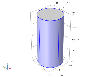
On the object , select Boundary 3 only.

It might be easier to select the correct boundary by using the window. To open this window, in the toolbar click and choose . (If you are running the cross-platform desktop, you find in the main menu.)

Click

Work Plane 1 (wp1)>Circle 1 (c1)

In the toolbar, click

In the window for , locate the section.

In the text field, type r0beam.

Click

Add Material

In the toolbar, click

to open the window.

Go to the window.

In the tree, select .

Click in the window toolbar.

In the toolbar, click

to close the window.

Definitions

Variables 1

In the toolbar, click

and choose .

In the window for , locate the section.

In the table, enter the following settings:


Name	Expression	Unit	Description
qr	sqrt(qx^2+qy^2)	m	Radial distance from beam axis
qrmax	cpt.max(qr)	m	Beam radius
z_avg	cpt.ave(qz)	m	Average z-coordinate
chi	qrmax/at(0,qrmax)		Ratio of beam radius to waist radius