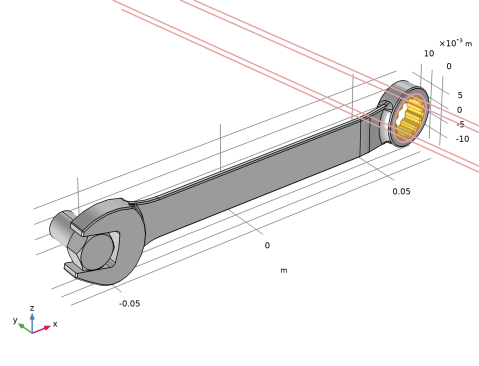
You are viewing the documentation for an older COMSOL version. The latest version is available here.
PDF

Shape Optimization of a Wrench
Introduction
Shape optimization can be used to alter the geometry of an existing product to improve its performance. This can be achieved using the Deformed Geometry interface, but one has to decide which shape deformations to allow. It is important to impose some restriction to preserve the mesh quality during the optimization. One approach is to use a Helmholtz filter to introduce a length scale, which (in combination with a Maximum displacement parameter) limits the slope of the shape variations. This type of regularized shape optimization can be setup using equations based modeling, but it is also built into the Free Shape Boundary feature. This model applies the feature to a CAD representation of a wrench, but the initial geometry can also come from topology optimization as shown in the model Shape Optimization of an MBB Beam.
Model Definition
Shape optimization is often subject to constraints on the geometry deformation, and in this model it does not make sense to deform the parts of the wrench that are designed to grab the bolt head. These parts are, however, associated with many boundaries, so the model uses two cylinder selections to define the fixed boundaries (Figure 1).
Figure 1: The plots shows one of the cylinder selections used to define the fixed boundaries. The selections are based on parameters that can be imported from a text file, but they can also be computed using the Measure functionality.
The wrench is made of structural steel and the objective is to maximize its stiffness without using more material. An initial study is performed to determine characteristic values for the total elastic strain energy and the volume. These values are used for scaling the optimization problem, which is an important step for constrained optimization problems.
Results and Discussion
Visualizing the shape deformation can require custom plots or tweaking of parameters for the default plot, but in this case the default plot shown in Figure 2 illustrates that
The two last points are a bit difficult to see, because the arrows are inside the geometry, but the relative normal boundary displacement is the displacement in the normal direction relative to the maximum possible displacement in the normal direction, so when this is significantly larger than zero and there are no arrows, it means that the arrows are inside the geometry. They can be seen by enabling transparency.
Figure 2: The default shape optimization plot shows the edges of the old geometry in gray together with a surface plot of the relative normal boundary displacement in colors. The actual displacement is shown with red arrows, but they are plotted inside the geometry wherever this is expanded.
Alternatively the initial and optimized volumes can be plotted on top of each other, but this plot only makes sense with transparency enabled. This plot is shown in Figure 3.This kind of plot can suffer from z-fighting artifacts on Symmetry/Roller boundaries, but this feature is not used in the model.
Figure 3: The shape of the wrench is optimized by removing material from the head and the handle. Furthermore, the middle part is thicker in the z direction and the kink near the handle has been straightened out.
Notes About the COMSOL Implementation
This model combines the Shape Optimization interface with the Solid Mechanics interfaces. First, you setup and solve the for the structural problem for the initial geometry. The objective and constraint can be defined automatically by using the study wizard, but you have to define the controls using the shape optimization features available on the component. Keep in mind that allowing a large Maximum displacement will result in NaN/Inf solver errors due to inverted elements.
Application Library path: Optimization_Module/Shape_Optimization/wrench_shape_optimization
Modeling Instructions
From the File menu, choose New.
New
In the New window, click  Model Wizard.
Model Wizard
1
In the Model Wizard window, click  3D.
2
In the Select Physics tree, select Structural Mechanics>Solid Mechanics (solid).
3
Click Add.
4
Click  Study.
5
In the Select Study tree, select Preset Studies for Selected Physics Interfaces>Optimization>Shape Optimization, Stationary.
6
Global Definitions
Geometrical Parameters
1
In the Home toolbar, click  Parameters and choose Add>Parameters.
2
In the Settings window for Parameters, type Geometrical Parameters in the Label text field.
Input the geometric parameters manually or load them from wrench_shape_optimization_parameters.txt. The parameters can be computed using the Measure geometry feature.
3
Locate the Parameters section. In the table, enter the following settings:
Geometry 1
Import 1 (imp1)
1
In the Home toolbar, click  Import.
2
In the Settings window for Import, locate the Import section.
3
Click  Browse.
4
5
Click  Import.
6
Locate the Selections of Resulting Entities section. Select the Resulting objects selection check box.
Nut Faces
1
In the Geometry toolbar, click  Selections and choose Cylinder Selection.
2
In the Settings window for Cylinder Selection, type Nut Faces in the Label text field.
3
Locate the Geometric Entity Level section. From the Level list, choose Boundary.
4
Locate the Size and Shape section. In the Outer radius text field, type dbolt*0.7.
5
Locate the Axis section. From the Axis type list, choose y-axis.
6
Locate the Position section. In the x text field, type xbolt.
7
In the y text field, type ybolt.
8
In the z text field, type zbolt.
9
Locate the Output Entities section. From the Include entity if list, choose Entity inside cylinder.
Handle Hole Faces
1
In the Geometry toolbar, click  Selections and choose Cylinder Selection.
2
In the Settings window for Cylinder Selection, type Handle Hole Faces in the Label text field.
3
Locate the Geometric Entity Level section. From the Level list, choose Boundary.
4
Locate the Size and Shape section. In the Outer radius text field, type dhole*0.6.
5
Locate the Position section. In the x text field, type xhole.
6
In the y text field, type yhole.
7
In the z text field, type zhole.
8
Locate the Axis section. From the Axis type list, choose Cartesian.
9
In the x text field, type xholeaxis.
10
In the y text field, type yholeaxis.
11
In the z text field, type zholeaxis.
12
Locate the Output Entities section. From the Include entity if list, choose Entity inside cylinder.
13
Click  Build Selected.
The selection should now look like that in Figure 1.
Interior Faces
1
In the Geometry toolbar, click  Selections and choose Adjacent Selection.
2
In the Settings window for Adjacent Selection, type Interior Faces in the Label text field.
3
Locate the Input Entities section. Click  Add.
4
In the Add dialog box, select Import 1 in the Input selections list.
5
Optimized Faces
1
In the Geometry toolbar, click  Selections and choose Complement Selection.
2
In the Settings window for Complement Selection, type Optimized Faces in the Label text field.
3
Locate the Geometric Entity Level section. From the Level list, choose Boundary.
4
Locate the Input Entities section. Click  Add.
5
In the Add dialog box, in the Selections to invert list, choose Nut Faces and Handle Hole Faces.
6
Add Material
1
In the Home toolbar, click  Add Material to open the Add Material window.
2
Go to the Add Material window.
3
In the tree, select Built-in>Structural steel.
4
Click Add to Component in the window toolbar.
5
In the Home toolbar, click  Add Material to close the Add Material window.
Solid Mechanics (solid)
Fixed Constraint 1
1
In the Model Builder window, under Component 1 (comp1) right-click Solid Mechanics (solid) and choose Fixed Constraint.
2
Boundary Load 1
1
In the Physics toolbar, click  Boundaries and choose Boundary Load.
2
3
In the Settings window for Boundary Load, locate the Force section.
4
From the Load type list, choose Total force.
5
Specify the Ftot vector as
Global Definitions
Parameters 1
1
In the Model Builder window, under Global Definitions click Parameters 1.
2
In the Settings window for Parameters, locate the Parameters section.
3
Mesh 1
1
In the Model Builder window, under Component 1 (comp1) click Mesh 1.
2
In the Settings window for Mesh, locate the Physics-Controlled Mesh section.
3
From the Element size list, choose Finer.
Shape Optimization
Free Shape Domain 1
Change the selection of the Free Shape Domain, so that the shape of the bolt is not changed.
1
In the Model Builder window, under Component 1 (comp1)>Shape Optimization click Free Shape Domain 1.
2
Definitions
Add a Free Shape Boundary feature to allow the shape of the wrench to change.
Component 1 (comp1)
Free Shape Boundary 1
1
In the Definitions toolbar, click  Optimization and choose Shape Optimization>Free Shape Boundary.
2
In the Settings window for Free Shape Boundary, locate the Boundary Selection section.
3
From the Selection list, choose Optimized Faces.
4
Locate the Control Variable Settings section. In the dmax text field, type maxD.
Study 1
Shape Optimization
1
In the Model Builder window, under Study 1 click Shape Optimization.
2
In the Settings window for Shape Optimization, locate the Optimization Solver section.
3
In the Move limits text field, type 0.2.
4
In the Maximum number of iterations text field, type 20.
5
From the Keep solutions list, choose Every Nth.
6
In the Save every Nth text field, type 21.
Setting a value larger than the maximum number of iterations, effectively saves the first and last iteration.
7
In the Model Builder window, click Study 1.
8
In the Settings window for Study, type Shape Optimization in the Label text field.
9
In the Study toolbar, click  Get Initial Value.
The deformed shape can be exported as an STL file.
10
In the Model Builder window, click Shape Optimization.
11
In the Settings window for Shape Optimization, locate the Output While Solving section.
12
Select the Plot check box.
13
From the Plot group list, choose Shape Optimization.
14
In the Study toolbar, click  Compute.
Results
Shape Optimization
1
In the Model Builder window, under Results click Shape Optimization.
2
In the Shape Optimization toolbar, click  Plot.
Mesh 1
1
In the Model Builder window, expand the Results>Datasets node.
2
Right-click Results>Datasets>Shape Optimization/Solution 1 (sol1) and choose Add Mesh to Export.
3
In the Settings window for Mesh, locate the Output section.
4
From the File type list, choose STL binary file (*.stl; *.STL).
5
In the Filename text field, type wrench_shape_optimization.stl.
Plot the initial and optimized volumes on top of each other to illustrate the shape change in a clear way (assuming transparency is enabled). This plot can give rise to z-fighting artifact on Symmetry/Roller boundaries, but this model does not use that feature.
Volumetric
1
In the Home toolbar, click  Add Plot Group and choose 3D Plot Group.
2
In the Settings window for 3D Plot Group, click to expand the Title section.
3
From the Title type list, choose Label.
4
In the Label text field, type Volumetric.
Optimized Design
1
Right-click Volumetric and choose Volume.
2
In the Settings window for Volume, type Optimized Design in the Label text field.
3
Locate the Coloring and Style section. From the Coloring list, choose Uniform.
Initial Design
1
Right-click Optimized Design and choose Duplicate.
2
In the Settings window for Volume, type Initial Design in the Label text field.
3
Locate the Data section. From the Dataset list, choose Shape Optimization/Solution 1 (sol1).
4
From the Optimization solution list, choose 0.
5
Locate the Coloring and Style section. From the Color list, choose Gray.
Line 1
1
In the Model Builder window, right-click Volumetric and choose Line.
2
In the Settings window for Line, locate the Data section.
3
From the Dataset list, choose Shape Optimization/Solution 1 (sol1).
4
From the Optimization solution list, choose 0.
5
Locate the Expression section. In the Expression text field, type 1.
6
Locate the Coloring and Style section. From the Coloring list, choose Uniform.
7
From the Color list, choose From theme.
8
Click the  Transparency button in the Graphics toolbar.
9
In the Volumetric toolbar, click  Plot.
Applied Loads (solid)
In the Model Builder window, under Results right-click Applied Loads (solid) and choose Delete.
Stress - Optimized Design
1
In the Model Builder window, under Results click Stress (solid).
2
In the Settings window for 3D Plot Group, type Stress - Optimized Design in the Label text field.