|
|
|


|
1
|
|
2
|
|
3
|
Click Add.
|
|
4
|
Click
|
|
5
|
|
6
|
Click
|
|
1
|
|
2
|
Browse to the model’s Application Libraries folder and double-click the file effective_diffusivity_geom_sequence.mph.
|
|
3
|
|
1
|
|
2
|
|
1
|
|
2
|
|
1
|
|
2
|
|
3
|
Clear the Convection check box.
|
|
1
|
In the Model Builder window, under Component 1 (comp1)>Transport of Diluted Species (tds) click Transport Properties 1.
|
|
2
|
|
3
|
|
1
|
|
2
|
|
3
|
|
1
|
|
2
|
|
3
|
|
4
|
|
5
|
|
1
|
|
2
|
|
3
|
|
4
|
|
5
|
|
6
|
|
1
|
|
2
|
|
3
|
|
4
|
|
1
|
|
2
|
|
1
|
|
2
|
|
3
|
|
4
|
|
5
|
|
1
|
|
2
|
|
3
|
|
4
|
|
6
|
|
7
|
|
1
|
|
2
|
|
3
|
|
4
|
|
5
|
|
1
|
|
2
|
|
3
|
|
4
|
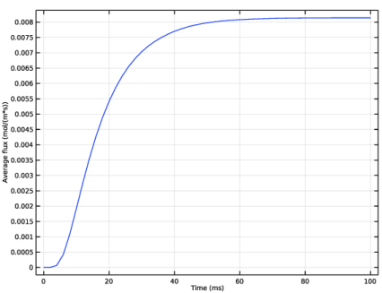
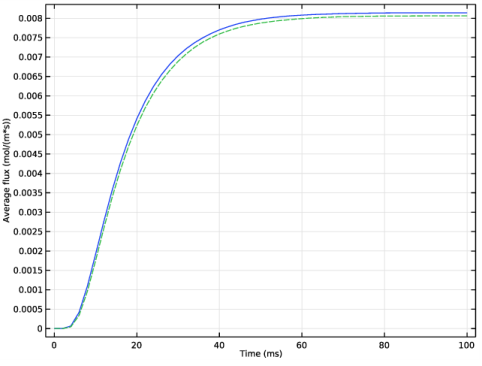
Click Replace Expression in the upper-right corner of the y-Axis Data section. From the menu, choose Component 1 (comp1)>Definitions>Variables>flux_avg - Average flux - mol/(m²·s).
|
|
1
|
|
2
|
|
3
|
|
4
|
|
5
|
|
6
|
|
7
|
|
1
|
|
2
|
|
3
|
|
4
|
Locate the Expressions section. In the table, enter the following settings:
|
|
5
|
Click
|
|
1
|
Go to the Table window.
|
|
1
|
|
2
|
|
3
|
|
4
|
Find the Physics interfaces in study subsection. In the table, clear the Solve check box for Study 1.
|
|
5
|
|
6
|
|
1
|
|
2
|
|
3
|
Find the Physics interfaces in study subsection. In the table, clear the Solve check box for Transport of Diluted Species (tds).
|
|
4
|
|
5
|
|
6
|
|
7
|
|
1
|
|
2
|
|
4
|
|
5
|
|
1
|
|
2
|
|
1
|
|
2
|
|
3
|
Clear the Convection check box.
|
|
1
|
In the Model Builder window, under Component 2 (comp2)>Transport of Diluted Species 2 (tds2) click Transport Properties 1.
|
|
2
|
|
3
|
|
1
|
|
2
|
|
3
|
|
1
|
|
3
|
|
4
|
|
5
|
|
1
|
|
3
|
|
4
|
|
5
|
|
6
|
|
1
|
|
2
|
|
1
|
|
2
|
|
3
|
|
4
|
|
1
|
|
2
|
|
3
|
|
4
|
|
5
|
|
1
|
|
2
|
|
3
|
|
5
|
Click Replace Expression in the upper-right corner of the y-Axis Data section. From the menu, choose Component 2 (comp2)>Definitions>Variables>flux_hom - Flux, 1D model - mol/(m²·s).
|
|
6
|
Click to expand the Coloring and Style section. Find the Line style subsection. From the Line list, choose Dashed.
|
|
7
|
|
1
|
|
2
|
|
3
|
|
4
|
|
5
|
|
6
|
Locate the Selections of Resulting Entities section. Select the Resulting objects selection check box.
|
|
7
|
|
1
|
|
2
|
|
3
|
|
4
|
|
5
|
|
1
|
|
2
|
Select the object fil1 only.
|
|
3
|
|
4
|
|
5
|
|
6
|
|
7
|
|
8
|
|
1
|
|
2
|
|
3
|
|
5
|
|
1
|
|
2
|
|
3
|
|
4
|
|
1
|
|
2
|
Select the object r1 only.
|
|
3
|
|
4
|
|
5
|
From the Objects to subtract list, choose Square 1 since the first square creates a Selection of Resulting Entities, all squares are included in this selection.
|
|
6
|
|
1
|
|
2
|
|
1
|
|
2
|
|
3
|
|
4
|
|
5
|
|
1
|
|
2
|
|
3
|
|
4
|
|
5
|
|
1
|
|
2
|
|
3
|
|
4
|
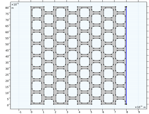
On the object fin, select Boundary 276 only.
|
|
5
|
|
6
|