PDF

Mechanism Submerged in Fluid
Introduction
Fluid-structure interaction (FSI) is a common class of multiphysics problems. The coupling is in general bidirectional; the fluid exerts an external load on the structure, leading to deformation of structural components, and, conversely, the motion or deformation of the structural components changes the flow field. Depending on the type of interaction between fluids and solid objects, FSI problems can be categorized as either one-way problems or fully coupled problems.
This example demonstrates the dynamics of a moving mechanism, with two rotating fins, submerged in a fluid channel. The fluid domain is modeled using the Laminar Flow interface, and the mechanism is modeled using the Multibody Dynamics interface. A Fluid-Structure Interaction, Pair multiphysics coupling is used to model the interaction between the fluid and solid domains, and an ALE formulation through a Moving Mesh node is used to control the geometrical changes of the fluid domain. A time-dependent study is used to simulate the forward motion of the mechanism through the fluid channel induced by the fin rotation.
Model Definition
The model geometry consists of a mechanism with a central body and two fins. The mechanism is submerged in a flow channel. The fins are located at the back of the body, symmetrically placed on both sides of the longitudinal axis at an initial angle of 30°. The fins are connected to the central body through hinge joints, which allow in-plane rotation of the fins, as shown in Figure 1. The mechanism is submerged in a flow channel of 25 cm width, 15 cm depth, and 5 cm height.
Figure 1: Geometry of the mechanism submerged in a fluid channel.
materials
The components of the mechanism are built of structural steel and the fluid around the mechanism is taken as water.
Fluid-Structure Interaction
The interaction between the fluid and the solid domains is modeled using a Fluid-Multibody Interaction, Assembly interface. This interface consists of a predefined Laminar Flow interface, a Multibody Dynamics interface, and a Moving Mesh node with a Deforming Domain subnode. In addition, a Multiphysics Couplings node is added. It contains the multiphysics coupling Fluid-Structure Interaction, Pair. Additional details about the interface can be found in the documentation for Multiphysics Couplings in the Multibody Dynamics Module User’s Guide.
The interaction between the fluid and the structural mechanism is specified through the interface boundaries between the two domains. The two identity pairs between the fluid and solid domains are selected in the Fluid-Structure Interaction, Pair node to incorporate the multiphysics coupling between the two physics.
Fluid Flow
The fluid in the channel is described by the incompressible Navier-Stokes equations for the velocity field and the pressure in the spatial (deformed) coordinate system. A Pressure Point Constraint is used at one of the corner points of the fluid domain, setting the value of the pressure to zero at this point.
MULTIBODY dynamics
The Multibody Dynamics interface is used to model the structural assembly. In this analysis, the solid central body is assumed to be a rigid object, while the fins are modeled as flexible bodies. The motion of the mechanism is initiated by a prescribed rotation of the fins about the central body in a time-dependent manner. The rotation is prescribed in such a way that during the initial 0.25 s, the fins rotate toward each other, resulting in the closing of the mechanism. After 0.25 s, their rotation is kept constant at 15°. Figure 7 shows the rotation of the fins as a function of time.
Moving mesh
The geometrical changes in the fluid domain are modeled using an ALE formulation. A deforming-domain condition is assigned to the fluid domain, where the shape of the domain is controlled by the moving boundaries and a smoothing equation in the interior. In the present example, two types of mesh boundary conditions are used to specify the motion of the spatial mesh:
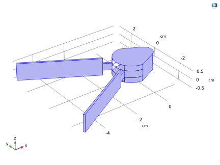
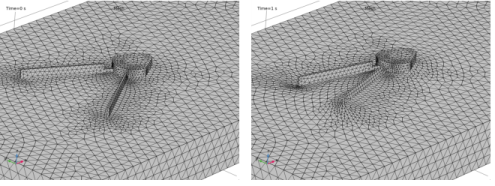
On all fluid-solid interface boundaries, except at the curved boundaries at the back of the solid body, a Prescribed Mesh Displacement boundary condition is used to transfer the motion of the adjoining solid to the moving mesh. As shown in Figure 2, this boundary condition sets the displacement of the mesh boundaries equal to the mapped solid boundaries of the identity pairs.
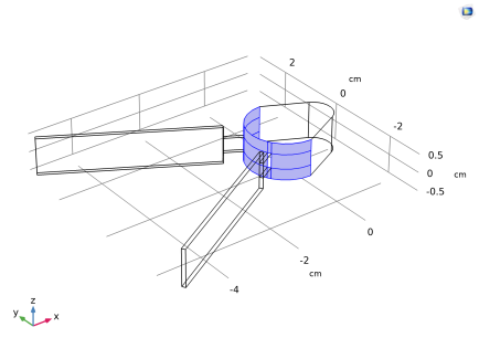
At the back side of the solid body as shown in Figure 3, the contact area between solid and fluid boundaries continuously changes because of the rotational motion of the fins. Using a Prescribed Normal Mesh Displacement boundary condition at these boundaries, allows the mesh to move freely in the tangential direction and to follow the solid normal motion in the normal direction.
Figure 2: Solid motion (all components) transferred to the moving mesh boundaries.
Figure 3: Normal component of solid motion transferred to the moving mesh boundaries. The mesh is free to slide in these boundaries in the tangential direction.
Study
A time dependent study is performed for 1 s to analyze the interaction of the mechanism and the fluid.
Results and Discussion
The velocity field and pressure distribution in the central xy-plane of the fluid domain are plotted in Figure 4 for six different time steps. Additionally, the variation of the structural displacement and velocity are plotted for each of these time steps. A similar plot for the distribution of the fluid velocity and pressure in the central xz-plane at t = 0.3 s is shown in Figure 5.
Figure 4: Velocity field (arrow) and pressure (surface) in the fluid in the xy-plane together with displacement (surface) and velocity (arrow) in the mechanism at different time steps.
The time-dependent rotational motion of the fins are shown in Figure 7. Initially, when the fins start to rotate and approach each other, they force the surrounding fluid either to compress or expand. After t = 0.25 s, the rotation of the fins are kept at a constant angle of 15°. The transmission of velocity from the structure to the fluid results in a net forward motion of the structure as shown in Figure 7.
Figure 5: Velocity field (arrow) and pressure (surface) in the fluid in the xz-plane together with displacement (surface) and velocity (arrow) in the mechanism at t = 0.3 s.
Figure 6 shows the finite-element mesh in the mechanism and the lower half of the fluid domain at the initial and final time steps. Because of the forward motion of the structure in the x direction, you can observe a stretching of the elements in this direction in the deformed mesh plot. If the displacements were even larger, remeshing would have to be considered.
Figure 6: Mesh at t = 0 and s.
Figure 7: Fin rotation and forward velocity of the mechanism as functions of time.
Notes About the COMSOL Implementation
The Fluid-Structure Interaction, Pair node operates on the geometry in the assembly state. Pairs between different geometry parts can then be automatically generated.
All the pairs in the geometry appear in the Pair Selection section of the Fluid-Structure Interaction, Pair node. Select only those pairs which couple the fluid and solid physics interfaces.
In order to transfer the deformation of the solid to the moving mesh, the built-in variables (fsip1.u_solid, fsip1.v_solid, and fsip1.w_solid) are available. These variables are equal to the solid displacement.
Application Library path: Multibody_Dynamics_Module/Tutorials/mechanism_submerged_in_fluid
Modeling Instructions
From the File menu, choose New.
New
In the New window, click  Model Wizard.
Model Wizard
1
In the Model Wizard window, click  3D.
2
In the Select Physics tree, select Fluid Flow>Fluid-Structure Interaction>Fluid-Multibody Interaction, Assembly.
3
Click Add.
4
Click  Study.
5
In the Select Study tree, select General Studies>Time Dependent.
6
Global Definitions
Parameters 1
1
In the Model Builder window, under Global Definitions click Parameters 1.
2
In the Settings window for Parameters, locate the Parameters section.
3
Geometry 1
1
In the Model Builder window, under Component 1 (comp1) click Geometry 1.
2
In the Settings window for Geometry, locate the Units section.
3
From the Length unit list, choose cm.
Import 1 (imp1)
You can import the geometry of the mechanism by browsing to the model’s Application Libraries folder.
1
In the Home toolbar, click  Import.
2
In the Settings window for Import, locate the Import section.
3
Click  Browse.
4
5
Click  Import.
Copy 1 (copy1)
1
In the Geometry toolbar, click  Transforms and choose Copy.
2
Click in the Graphics window and then press Ctrl+A to select both objects.
3
In the Settings window for Copy, click  Build Selected.
Block 1 (blk1)
1
In the Geometry toolbar, click  Block.
2
In the Settings window for Block, locate the Size and Shape section.
3
In the Width text field, type 25.
4
In the Depth text field, type 15.
5
In the Height text field, type 5.
6
Locate the Position section. From the Base list, choose Center.
7
Click  Build Selected.
Work Plane 1 (wp1)
1
In the Geometry toolbar, click  Work Plane.
2
In the Settings window for Work Plane, click  Build Selected.
Work Plane 2 (wp2)
1
Right-click Work Plane 1 (wp1) and choose Duplicate.
2
In the Settings window for Work Plane, locate the Plane Definition section.
3
From the Plane list, choose xz-plane.
4
Click  Build Selected.
Partition Domains 1 (pard1)
1
In the Geometry toolbar, click  Booleans and Partitions and choose Partition Domains.
2
On the object blk1, select Domain 1 only.
3
In the Settings window for Partition Domains, locate the Partition Domains section.
4
From the Work plane list, choose Work Plane 1 (wp1).
5
Click  Build Selected.
Partition Domains 2 (pard2)
1
Right-click Partition Domains 1 (pard1) and choose Duplicate.
2
On the object pard1, select Domains 1 and 2 only.
3
In the Settings window for Partition Domains, locate the Partition Domains section.
4
From the Work plane list, choose Work Plane 2 (wp2).
5
Click  Build Selected.
Difference 1 (dif1)
1
In the Geometry toolbar, click  Booleans and Partitions and choose Difference.
2
3
In the Settings window for Difference, locate the Difference section.
4
Find the Objects to subtract subsection. Click to select the  Activate Selection toggle button.
5
Select the objects copy1(1) and copy1(2) only.
6
Click  Build Selected.
Form Union (fin)
1
In the Model Builder window, under Component 1 (comp1)>Geometry 1 click Form Union (fin).
2
In the Settings window for Form Union/Assembly, locate the Form Union/Assembly section.
3
From the Action list, choose Form an assembly.
4
Click  Build Selected.
For better visualization, you can hide the top part of the fluid domain and view the mechanism using wireframe rendering.
5
In the Model Builder window, click Geometry 1.
6
Click the  Click and Hide button in the Graphics toolbar.
7
In the Graphics window toolbar, clicknext to  Select Objects, then choose Select Domains.
8
On the object fin, select Domains 2 and 4 only.
9
Click the  Wireframe Rendering button in the Graphics toolbar.
Definitions
Step 1 (step1)
1
In the Home toolbar, click  Functions and choose Global>Step.
2
In the Settings window for Step, click to expand the Smoothing section.
3
Locate the Parameters section. In the Location text field, type 0.05[s].
Analytic 1 (an1)
1
In the Home toolbar, click  Functions and choose Global>Analytic.
2
In the Settings window for Analytic, locate the Definition section.
3
In the Expression text field, type th_max*(sin(2*pi*1*t)*(t<0.25)*step1(t)+(t>=0.25)).
4
In the Arguments text field, type t.
5
Locate the Units section. In the table, enter the following settings:
6
In the Function text field, type rad.
Variables 1
1
In the Model Builder window, right-click Definitions and choose Variables.
2
In the Settings window for Variables, locate the Variables section.
3
Identity Boundary Pair 1 (ap1)
You can group the interface boundaries by creating selections from the source and destination boundaries of the identity pairs. To identify the boundaries of each domain of the assembly, you can hide one of the domains and use selection highlights to see the boundaries of the unhidden domain.
1
In the Model Builder window, click Identity Boundary Pair 1 (ap1).
2
In the Settings window for Pair, locate the Source Boundaries section.
3
Click  Create Selection.
4
In the Create Selection dialog box, type Fluid Boundaries (Fins) in the Selection name text field.
5
6
In the Settings window for Pair, locate the Destination Boundaries section.
7
Click  Create Selection.
8
In the Create Selection dialog box, type Solid Boundaries(Fins) in the Selection name text field.
9
10
In the Settings window for Pair, locate the Frame section.
11
From the Source frame list, choose Material  (X, Y, Z).
12
From the Destination frame list, choose Material  (X, Y, Z).
Identity Boundary Pair 2 (ap2)
1
In the Model Builder window, click Identity Boundary Pair 2 (ap2).
2
In the Settings window for Pair, locate the Source Boundaries section.
3
Click  Create Selection.
4
In the Create Selection dialog box, type Fluid Boundaries (Body) in the Selection name text field.
5
6
In the Settings window for Pair, locate the Destination Boundaries section.
7
Click  Create Selection.
8
In the Create Selection dialog box, type Solid Boundaries (Body) in the Selection name text field.
9
10
In the Settings window for Pair, locate the Frame section.
11
From the Source frame list, choose Material  (X, Y, Z).
12
From the Destination frame list, choose Material  (X, Y, Z).
All Fluid Boundaries
1
In the Definitions toolbar, click  Union.
2
In the Settings window for Union, type All Fluid Boundaries in the Label text field.
3
Locate the Geometric Entity Level section. From the Level list, choose Boundary.
4
Locate the Input Entities section. Under Selections to add, click  Add.
5
In the Add dialog box, in the Selections to add list, choose Fluid Boundaries (Fins) and Fluid Boundaries (Body).
6
Sliding Mesh Boundaries
1
In the Model Builder window, right-click Fluid Boundaries (Fins) and choose Duplicate.
2
In the Settings window for Explicit, type Sliding Mesh Boundaries in the Label text field.
3
Locate the Input Entities section. Click  Clear Selection.
4
Modify the domain selections and apply boundary conditions to the Laminar Flow and Multibody Dynamics physics interfaces.
Laminar Flow (spf)
1
In the Model Builder window, under Component 1 (comp1) click Laminar Flow (spf).
2
In the Settings window for Laminar Flow, locate the Domain Selection section.
3
4
Click  Remove from Selection.
5
Wall 1
1
In the Model Builder window, under Component 1 (comp1)>Laminar Flow (spf) click Wall 1.
2
In the Settings window for Wall, locate the Boundary Condition section.
3
From the Wall condition list, choose Slip.
Pressure Point Constraint 1
1
In the Physics toolbar, click  Points and choose Pressure Point Constraint.
2
Multibody Dynamics (mbd)
1
In the Model Builder window, under Component 1 (comp1) click Multibody Dynamics (mbd).
2
Rigid Material: Body
1
In the Physics toolbar, click  Domains and choose Rigid Material.
2
In the Settings window for Rigid Material, type Rigid Material: Body in the Label text field.
3
Attachment: Fin 1
1
In the Physics toolbar, click  Boundaries and choose Attachment.
2
In the Settings window for Attachment, type Attachment: Fin 1 in the Label text field.
3
Attachment: Fin 2
1
Right-click Attachment: Fin 1 and choose Duplicate.
2
In the Settings window for Attachment, type Attachment: Fin 2 in the Label text field.
3
Locate the Boundary Selection section. Click  Clear Selection.
4
Hinge Joint 1
1
In the Physics toolbar, click  Global and choose Hinge Joint.
2
In the Settings window for Hinge Joint, locate the Attachment Selection section.
3
From the Source list, choose Rigid Material: Body.
4
From the Destination list, choose Attachment: Fin 1.
5
Locate the Center of Joint section. From the list, choose User defined.
6
Locate the Axis of Joint section. Specify the e0 vector as
Prescribed Motion 1
1
In the Physics toolbar, click  Attributes and choose Prescribed Motion.
2
In the Settings window for Prescribed Motion, locate the Prescribed Rotational Motion section.
3
In the θp text field, type -th.
Hinge Joint 2
1
In the Model Builder window, under Component 1 (comp1)>Multibody Dynamics (mbd) right-click Hinge Joint 1 and choose Duplicate.
2
In the Settings window for Hinge Joint, locate the Attachment Selection section.
3
From the Destination list, choose Attachment: Fin 2.
Prescribed Motion 1
1
In the Model Builder window, expand the Hinge Joint 2 node, then click Prescribed Motion 1.
2
In the Settings window for Prescribed Motion, locate the Prescribed Rotational Motion section.
3
In the θp text field, type th.
Now you can add the moving mesh to the fluid domain.
Moving Mesh
Deforming Domain 1
1
In the Model Builder window, under Component 1 (comp1)>Moving Mesh click Deforming Domain 1.
2
Component 1 (comp1)
Prescribed Mesh Displacement 1
1
In the Definitions toolbar, click  Moving Mesh and choose Boundaries>Prescribed Mesh Displacement.
2
In the Settings window for Prescribed Mesh Displacement, locate the Boundary Selection section.
3
From the Selection list, choose All Fluid Boundaries.
4
Locate the Prescribed Mesh Displacement section. Specify the dx vector as
Prescribed Normal Mesh Displacement 1
1
In the Definitions toolbar, click  Moving Mesh and choose Boundaries>Prescribed Normal Mesh Displacement.
2
In the Settings window for Prescribed Normal Mesh Displacement, locate the Boundary Selection section.
3
From the Selection list, choose Sliding Mesh Boundaries.
4
Locate the Prescribed Normal Mesh Displacement section. In the dn text field, type un_solid.
5
Click to expand the Constraint Settings section. From the Constraint type list, choose Nitsche method.
After assigning physics interfaces to all the domains, add materials to the domains.
Add Material
1
In the Home toolbar, click  Add Material to open the Add Material window.
2
Go to the Add Material window.
3
In the tree, select Built-in>Water, liquid.
4
Click Add to Component in the window toolbar.
5
In the tree, select Built-in>Structural steel.
6
Click Add to Component in the window toolbar.
Materials
Water, liquid (mat1)
1
In the Model Builder window, under Component 1 (comp1)>Materials click Water, liquid (mat1).
2
In the Settings window for Material, locate the Geometric Entity Selection section.
3
4
Click  Remove from Selection.
5
Structural steel (mat2)
1
In the Model Builder window, click Structural steel (mat2).
2
3
In the Home toolbar, click  Add Material to close the Add Material window.
Mesh 1
1
In the Settings window for Mesh, locate the Physics-Controlled Mesh section.
2
From the Element size list, choose Fine.
Size
Right-click Component 1 (comp1)>Mesh 1 and choose Edit Physics-Induced Sequence.
Size 2
1
In the Settings window for Size, locate the Geometric Entity Selection section.
2
From the Selection list, choose Solid Boundaries (Body).
3
Locate the Element Size section. From the Predefined list, choose Fine.
4
In the Model Builder window, right-click Mesh 1 and choose Build All.
Multiphysics
You can choose the pairs on which fluid-structure interaction occurs.
Fluid-Structure Interaction, Pair 1 (fsip1)
1
In the Model Builder window, under Component 1 (comp1)>Multiphysics click Fluid-Structure Interaction, Pair 1 (fsip1).
2
In the Settings window for Fluid-Structure Interaction, Pair, locate the Pair Selection section.
3
Under Pairs, click  Add.
4
In the Add dialog box, in the Pairs list, choose Identity Boundary Pair 1 (ap1) and Identity Boundary Pair 2 (ap2).
5
Study 1
Step 1: Time Dependent
1
In the Model Builder window, under Study 1 click Step 1: Time Dependent.
2
In the Settings window for Time Dependent, locate the Study Settings section.
3
In the Output times text field, type range(0,0.01,0.3) range(0.32,0.02,1).
4
From the Tolerance list, choose User controlled.
5
In the Relative tolerance text field, type 0.005.
Solution 1 (sol1)
1
In the Study toolbar, click  Show Default Solver.
2
In the Model Builder window, expand the Solution 1 (sol1) node, then click Time-Dependent Solver 1.
3
In the Settings window for Time-Dependent Solver, click to expand the Time Stepping section.
4
From the Steps taken by solver list, choose Intermediate.
5
Find the Algebraic variable settings subsection. In the Fraction of initial step for Backward Euler text field, type 0.01.
6
In the Model Builder window, expand the Study 1>Solver Configurations>Solution 1 (sol1)>Time-Dependent Solver 1>Segregated 1 node, then click Displacement field.
7
In the Settings window for Segregated Step, click to expand the Method and Termination section.
8
From the Jacobian update list, choose On every iteration.
Step 1: Time Dependent
1
In the Model Builder window, under Study 1 right-click Step 1: Time Dependent and choose Get Initial Value for Step.
2
In the Settings window for Time Dependent, click to expand the Results While Solving section.
3
Select the Plot check box.
4
From the Plot group list, choose Displacement (mbd).
5
In the Study toolbar, click  Compute.
Results
Velocity (spf)
1
In the Settings window for 3D Plot Group, locate the Data section.
2
From the Time (s) list, choose 1.
3
In the Velocity (spf) toolbar, click  Plot.
Pressure (spf)
1
In the Model Builder window, click Pressure (spf).
2
In the Settings window for 3D Plot Group, locate the Data section.
3
From the Time (s) list, choose 1.
4
In the Pressure (spf) toolbar, click  Plot.
Velocity (mbd)
1
In the Model Builder window, click Velocity (mbd).
2
In the Settings window for 3D Plot Group, locate the Data section.
3
From the Time (s) list, choose 1.
Arrow Line
1
In the Model Builder window, expand the Velocity (mbd) node, then click Arrow Line.
2
In the Settings window for Arrow Line, locate the Coloring and Style section.
3
Select the Scale factor check box. In the associated text field, type 35.
4
Locate the Arrow Positioning section. From the Placement list, choose Uniform.
5
In the Number of arrows text field, type 4000.
6
Locate the Coloring and Style section. From the Color list, choose Cyan.
7
In the Velocity (mbd) toolbar, click  Plot.
Displacement (mbd), Pressure (spf), Velocity (mbd), Velocity (spf)
1
In the Model Builder window, under Results, Ctrl-click to select Velocity (spf), Pressure (spf), Displacement (mbd), and Velocity (mbd).
2
Default Plots
In the Settings window for Group, type Default Plots in the Label text field.
For better visualization of the results, you can also set a new view of the assembly.
Fluid Pressure (xy) & Solid Displacement
Follow the instructions below to plot the fluid velocity and pressure fields in the xy-plane as well as the displacement and velocity of the mechanism. Compare the resulting plot with the one shown in Figure 4.
1
In the Home toolbar, click  Add Plot Group and choose 3D Plot Group.
2
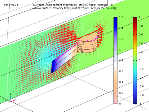
In the Settings window for 3D Plot Group, type Fluid Pressure (xy) & Solid Displacement in the Label text field.
3
Locate the Data section. From the Time (s) list, choose 0.3.
4
Locate the Plot Settings section. From the Frame list, choose Spatial  (x, y, z).
Solid Displacement
1
Right-click Fluid Pressure (xy) & Solid Displacement and choose Surface.
2
In the Settings window for Surface, type Solid Displacement in the Label text field.
3
Click Replace Expression in the upper-right corner of the Expression section. From the menu, choose Component 1 (comp1)>Multibody Dynamics>Displacement>mbd.disp - Displacement magnitude - m.
4
Click to expand the Range section. Select the Manual color range check box.
5
In the Maximum text field, type 1.6.
6
Locate the Coloring and Style section. Click  Change Color Table.
7
In the Color Table dialog box, select Aurora>Twilight in the tree.
8
Pressure
1
Right-click Solid Displacement and choose Duplicate.
2
In the Settings window for Surface, type Pressure in the Label text field.
3
Click Replace Expression in the upper-right corner of the Expression section. From the menu, choose Component 1 (comp1)>Laminar Flow>Velocity and pressure>p - Pressure - Pa.
4
Locate the Range section. In the Minimum text field, type -1.
5
In the Maximum text field, type 1.
6
Locate the Coloring and Style section. Click  Change Color Table.
7
In the Color Table dialog box, select Rainbow>Rainbow in the tree.
8
Selection 1
1
Right-click Pressure and choose Selection.
2
Pressure Contour
1
In the Model Builder window, right-click Fluid Pressure (xy) & Solid Displacement and choose Contour.
2
In the Settings window for Contour, type Pressure Contour in the Label text field.
3
Click Replace Expression in the upper-right corner of the Expression section. From the menu, choose Component 1 (comp1)>Laminar Flow>Velocity and pressure>p - Pressure - Pa.
4
Click to expand the Title section. From the Title type list, choose None.
5
Locate the Coloring and Style section. From the Coloring list, choose Uniform.
6
From the Color list, choose White.
7
Clear the Color legend check box.
Selection 1
1
Right-click Pressure Contour and choose Selection.
2
Fluid Velocity
1
In the Model Builder window, right-click Fluid Pressure (xy) & Solid Displacement and choose Arrow Surface.
2
In the Settings window for Arrow Surface, type Fluid Velocity in the Label text field.
3
Locate the Coloring and Style section.
4
Select the Scale factor check box. In the associated text field, type 20.
5
Locate the Arrow Positioning section. In the Number of arrows text field, type 4000.
Selection 1
1
Right-click Fluid Velocity and choose Selection.
2
Solid Velocity
1
In the Model Builder window, right-click Fluid Pressure (xy) & Solid Displacement and choose Arrow Line.
2
In the Settings window for Arrow Line, type Solid Velocity in the Label text field.
3
Click Replace Expression in the upper-right corner of the Expression section. From the menu, choose Component 1 (comp1)>Multibody Dynamics>Acceleration and velocity>mbd.u_tX,mbd.u_tY,mbd.u_tZ - Velocity.
4
Locate the Coloring and Style section.
5
Select the Scale factor check box. In the associated text field, type 35.
6
Locate the Arrow Positioning section. In the Number of arrows text field, type 50.
7
Locate the Coloring and Style section. From the Color list, choose Magenta.
Selection 1
1
Right-click Solid Velocity and choose Selection.
2
3
In the Fluid Pressure (xy) & Solid Displacement toolbar, click  Plot.
Fluid Pressure (xz) & Solid Displacement
Follow the instructions below to plot the fluid velocity and pressure fields in the xz-plane as well as the displacement and velocity of the mechanism. Compare the resulting plot with the one shown in Figure 5.
1
Right-click Selection 1 and choose Duplicate.
2
In the Settings window for 3D Plot Group, type Fluid Pressure (xz) & Solid Displacement in the Label text field.
3
In the Model Builder window, expand the Fluid Pressure (xz) & Solid Displacement node.
Selection 1
1
In the Model Builder window, expand the Results>Fluid Pressure (xz) & Solid Displacement>Pressure node, then click Selection 1.
2
In the Settings window for Selection, locate the Selection section.
3
Click  Clear Selection.
4
Click  Paste Selection.
5
In the Paste Selection dialog box, type 9 12 in the Selection text field.
6
Selection 1
1
In the Model Builder window, expand the Results>Fluid Pressure (xz) & Solid Displacement>Pressure Contour node, then click Selection 1.
2
In the Settings window for Selection, locate the Selection section.
3
Click  Clear Selection.
4
Click  Paste Selection.
5
In the Paste Selection dialog box, type 9 12 in the Selection text field.
6
Fluid Velocity
1
In the Model Builder window, under Results>Fluid Pressure (xz) & Solid Displacement click Fluid Velocity.
2
In the Settings window for Arrow Surface, locate the Coloring and Style section.
3
In the Scale factor text field, type 100.
Selection 1
1
In the Model Builder window, expand the Fluid Velocity node, then click Selection 1.
2
In the Settings window for Selection, locate the Selection section.
3
Click  Clear Selection.
4
Click  Paste Selection.
5
In the Paste Selection dialog box, type 9 12 in the Selection text field.
6
7
In the Fluid Pressure (xz) & Solid Displacement toolbar, click  Plot.
Follow the instructions below to plot the deformed mesh. The resulting plot should match the one shown in Figure 6.
Deformed Mesh
1
In the Home toolbar, click  Add Plot Group and choose 3D Plot Group.
2
In the Settings window for 3D Plot Group, type Deformed Mesh in the Label text field.
3
Locate the Plot Settings section. From the Frame list, choose Spatial  (x, y, z).
Mesh 1
1
Right-click Deformed Mesh and choose Mesh.
2
In the Settings window for Mesh, locate the Level section.
3
From the Level list, choose Volume.
4
Locate the Coloring and Style section. From the Element color list, choose Gray.
5
In the Deformed Mesh toolbar, click  Plot.
Follow the instructions below to plot the fin rotations and forward velocity of the structure. The resulting plot should match the one shown in Figure 7.
1D Plot Group 8
In the Home toolbar, click  Add Plot Group and choose 1D Plot Group.
Fin Rotation
1
Right-click 1D Plot Group 8 and choose Global.
2
In the Settings window for Global, type Fin Rotation in the Label text field.
3
Locate the y-Axis Data section. In the table, enter the following settings:
Fin Rotation 1
Right-click Fin Rotation and choose Duplicate.
Forward velocity
1
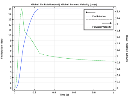
In the Model Builder window, expand the Results>1D Plot Group 8>Fin Rotation node, then click Results>1D Plot Group 8>Fin Rotation 1.
2
In the Settings window for Global, type Forward velocity in the Label text field.
3
Locate the y-Axis Data section. In the table, enter the following settings:
4
Click to expand the Coloring and Style section. Find the Line style subsection. From the Line list, choose Dashed.
Fin Rotation & Velocity
1
In the Model Builder window, under Results click 1D Plot Group 8.
2
In the Settings window for 1D Plot Group, type Fin Rotation & Velocity in the Label text field.
3
Locate the Plot Settings section.
4
Select the y-axis label check box. In the associated text field, type Fin Rotation (deg).
5
Select the Two y-axes check box.
6
In the table, select the Plot on secondary y-axis check box for Forward velocity.
Fluid Pressure (xy) & Solid Displacement
1
In the Results toolbar, click  Animation and choose Player.
2
In the Settings window for Animation, type Fluid Pressure (xy) & Solid Displacement in the Label text field.
3
Locate the Scene section. From the Subject list, choose Fluid Pressure (xy) & Solid Displacement.
4
Click the  Play button in the Graphics toolbar.
Fluid Pressure (xz) & Solid Displacement
1
Right-click Fluid Pressure (xy) & Solid Displacement and choose Duplicate.
2
In the Settings window for Animation, type Fluid Pressure (xz) & Solid Displacement in the Label text field.
3
Locate the Scene section. From the Subject list, choose Fluid Pressure (xz) & Solid Displacement.
4
Click the  Play button in the Graphics toolbar.
Deformed Mesh
1
Right-click Fluid Pressure (xz) & Solid Displacement and choose Duplicate.
2
In the Settings window for Animation, type Deformed Mesh in the Label text field.
3
Locate the Scene section. From the Subject list, choose Deformed Mesh.
4
Click the  Play button in the Graphics toolbar.