|
|
|
|
•
|
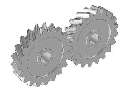
To build a gear geometry, you can import a gear part from the Parts Library and customize it by changing its input parameters. Alternatively, you can also create an equivalent disc or cone to represent the gear.
|
|
•
|
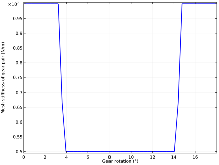
All the gears are assumed rigid. The elasticity of a gear mesh can be included in the Gear Pair nodes using the Gear Elasticity subnode.
|
|
•
|
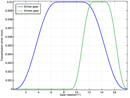
All the Gear Pair nodes are assumed ideal and frictionless. You can add Transmission Error, Backlash, or Friction subnodes when required.
|
|
•
|
To constraint the motion of a gear, you can use Prescribed Displacement/Rotation or Fixed Constraint subnodes. Alternatively, you can mount the gears on a shaft or on the ground through various Joint nodes.
|
|
•
|
The contact force on a Gear Pair is computed using Weak constraints or Penalty method. By default, the contact force computation is turned off. Use the weak constraints method for more accurate contact forces. However, you preferably opt for the penalty method for large rigid body systems.
|
|
1
|
|
2
|
|
3
|
Click Add.
|
|
4
|
Click
|
|
5
|
|
6
|
Click
|
|
1
|
|
2
|
|
3
|
|
4
|
Browse to the model’s Application Libraries folder and double-click the file helical_gear_pair_parameters.txt.
|
|
1
|
|
2
|
In the Part Libraries window, select Multibody Dynamics Module>3D>External Gears>helical_gear in the tree.
|
|
3
|
|
1
|
|
2
|
|
3
|
|
1
|
|
2
|
|
1
|
|
2
|
|
3
|
|
4
|
|
5
|
|
1
|
|
2
|
|
3
|
|
4
|
|
5
|
|
1
|
|
2
|
|
3
|
|
4
|
|
5
|
|
1
|
|
2
|
|
3
|
|
4
|
|
5
|
|
1
|
|
2
|
In the Settings window for Multibody Dynamics, click Physics Node Generation in the upper-right corner of the Automated Model Setup section. From the menu, choose Create Gears.
|
|
1
|
|
2
|
|
3
|
|
1
|
|
2
|
|
3
|
Specify the ω vector as
|
|
1
|
In the Model Builder window, expand the Component 1 (comp1)>Multibody Dynamics (mbd)>Gears>Helical Gear 2 node, then click Helical Gear 2.
|
|
2
|
|
3
|
|
4
|
|
1
|
|
2
|
|
3
|
Specify the ω vector as
|
|
1
|
|
2
|
|
3
|
|
4
|
|
5
|
|
1
|
|
2
|
|
3
|
|
1
|
|
2
|
In the Settings window for Hinge Joint, type Hinge Joint: Fixed-Gear 2 (Elastic) in the Label text field.
|
|
3
|
|
1
|
|
2
|
|
3
|
|
4
|
|
1
|
In the Model Builder window, under Component 1 (comp1)>Multibody Dynamics (mbd) click Hinge Joint: Fixed-Gear 1.
|
|
1
|
|
2
|
|
3
|
|
4
|
|
1
|
|
2
|
|
3
|
From the list, choose Joint.
|
|
4
|
|
1
|
|
2
|
|
3
|
|
4
|
|
5
|
Locate the Contact Force Computation section. From the list, choose Computed using weak constraints.
|
|
1
|
|
2
|
|
3
|
|
1
|
|
2
|
|
1
|
|
2
|
|
3
|
|
1
|
In the Model Builder window, under Component 1 (comp1)>Multibody Dynamics (mbd)>Gear Pair: Constant Stiffness click Gear Elasticity 1.
|
|
2
|
|
3
|
|
4
|
|
5
|
|
1
|
In the Model Builder window, expand the Component 1 (comp1)>Multibody Dynamics (mbd)>Gear Pair: Varying Stiffness node, then click Gear Elasticity 1.
|
|
2
|
|
3
|
|
4
|
|
5
|
|
6
|
|
7
|
|
1
|
In the Model Builder window, under Component 1 (comp1)>Multibody Dynamics (mbd)>Gear Pair: Transmission Error click Gear Elasticity 1.
|
|
2
|
|
3
|
|
4
|
|
5
|
|
1
|
|
2
|
|
3
|
|
4
|
|
1
|
|
2
|
|
3
|
|
1
|
|
2
|
|
3
|
|
4
|
|
5
|
|
6
|
Locate the Physics and Variables Selection section. Select the Modify model configuration for study step check box.
|
|
7
|
In the tree, select Component 1 (comp1)>Multibody Dynamics (mbd), Controls spatial frame>Hinge Joint: Fixed-Gear 2 (Elastic), Component 1 (comp1)>Multibody Dynamics (mbd), Controls spatial frame>Gear Pair: Constant Stiffness, Component 1 (comp1)>Multibody Dynamics (mbd), Controls spatial frame>Gear Pair: Varying Stiffness, and Component 1 (comp1)>Multibody Dynamics (mbd), Controls spatial frame>Gear Pair: Transmission Error.
|
|
8
|
Click
|
|
1
|
|
2
|
|
3
|
|
4
|
|
5
|
|
1
|
|
2
|
|
3
|
|
4
|
|
5
|
|
1
|
|
2
|
In the Settings window for Study, type Study 2: Transient (Constant Stiffness) in the Label text field.
|
|
3
|
|
1
|
In the Model Builder window, under Study 2: Transient (Constant Stiffness) click Step 1: Time Dependent.
|
|
2
|
|
3
|
|
4
|
|
5
|
|
6
|
Locate the Physics and Variables Selection section. Select the Modify model configuration for study step check box.
|
|
7
|
In the tree, select Component 1 (comp1)>Multibody Dynamics (mbd), Controls spatial frame>Hinge Joint: Fixed-Gear 2 (Elastic), Component 1 (comp1)>Multibody Dynamics (mbd), Controls spatial frame>Gear Pair: Rigid, Component 1 (comp1)>Multibody Dynamics (mbd), Controls spatial frame>Gear Pair: Varying Stiffness, and Component 1 (comp1)>Multibody Dynamics (mbd), Controls spatial frame>Gear Pair: Transmission Error.
|
|
8
|
Click
|
|
1
|
|
2
|
|
3
|
|
4
|
|
5
|
|
1
|
|
2
|
|
3
|
|
4
|
|
5
|
|
1
|
|
2
|
In the Settings window for Study, type Study 3: Transient (Varying Stiffness) in the Label text field.
|
|
3
|
|
1
|
In the Model Builder window, under Study 3: Transient (Varying Stiffness) click Step 1: Time Dependent.
|
|
2
|
|
3
|
|
4
|
|
5
|
|
6
|
Locate the Physics and Variables Selection section. Select the Modify model configuration for study step check box.
|
|
7
|
In the tree, select Component 1 (comp1)>Multibody Dynamics (mbd), Controls spatial frame>Hinge Joint: Fixed-Gear 2 (Elastic), Component 1 (comp1)>Multibody Dynamics (mbd), Controls spatial frame>Gear Pair: Rigid, Component 1 (comp1)>Multibody Dynamics (mbd), Controls spatial frame>Gear Pair: Constant Stiffness, and Component 1 (comp1)>Multibody Dynamics (mbd), Controls spatial frame>Gear Pair: Transmission Error.
|
|
8
|
Click
|
|
1
|
|
2
|
|
3
|
|
4
|
|
5
|
|
1
|
|
2
|
|
3
|
|
4
|
|
5
|
|
1
|
|
2
|
In the Settings window for Study, type Study 4: Transient (Transmission Error) in the Label text field.
|
|
3
|
|
1
|
In the Model Builder window, under Study 4: Transient (Transmission Error) click Step 1: Time Dependent.
|
|
2
|
|
3
|
|
4
|
|
5
|
|
6
|
Locate the Physics and Variables Selection section. Select the Modify model configuration for study step check box.
|
|
7
|
In the tree, select Component 1 (comp1)>Multibody Dynamics (mbd), Controls spatial frame>Hinge Joint: Fixed-Gear 2 (Elastic), Component 1 (comp1)>Multibody Dynamics (mbd), Controls spatial frame>Gear Pair: Rigid, Component 1 (comp1)>Multibody Dynamics (mbd), Controls spatial frame>Gear Pair: Constant Stiffness, and Component 1 (comp1)>Multibody Dynamics (mbd), Controls spatial frame>Gear Pair: Varying Stiffness.
|
|
8
|
Click
|
|
1
|
|
2
|
|
3
|
|
4
|
|
5
|
|
1
|
|
2
|
|
3
|
|
4
|
|
5
|
|
1
|
|
2
|
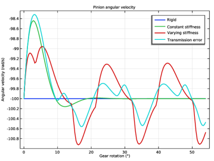
In the Settings window for Global, click Replace Expression in the upper-right corner of the y-Axis Data section. From the menu, choose Component 1 (comp1)>Multibody Dynamics>Gear pairs>Gear Pair: Rigid>Pinion>mbd.grp1.tht_pn - Pinion angular velocity - rad/s.
|
|
3
|
|
4
|
Click Replace Expression in the upper-right corner of the x-Axis Data section. From the menu, choose Component 1 (comp1)>Multibody Dynamics>Hinge joints>Hinge Joint: Fixed-Gear 1>mbd.hgj1.th - Relative rotation - rad.
|
|
5
|
|
6
|
|
7
|
|
8
|
|
1
|
|
2
|
|
3
|
|
4
|
|
5
|
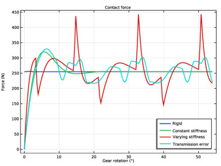
Locate the Data section. From the Dataset list, choose Study 2: Transient (Constant Stiffness)/Solution 2 (sol2).
|
|
6
|
Locate the Legends section. In the table, enter the following settings:
|
|
1
|
|
2
|
|
3
|
|
4
|
|
5
|
Locate the Data section. From the Dataset list, choose Study 3: Transient (Varying Stiffness)/Solution 3 (sol3).
|
|
6
|
Locate the Legends section. In the table, enter the following settings:
|
|
1
|
|
2
|
|
3
|
|
4
|
|
5
|
Locate the Data section. From the Dataset list, choose Study 4: Transient (Transmission Error)/Solution 4 (sol4).
|
|
6
|
Locate the Legends section. In the table, enter the following settings:
|
|
1
|
|
2
|
|
3
|
|
1
|
|
2
|
|
3
|
|
4
|
|
1
|
|
2
|
|
1
|
|
2
|
|
1
|
|
2
|
|
1
|
|
2
|
|
4
|
|
5
|
|
1
|
|
2
|
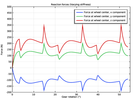
In the Settings window for 1D Plot Group, type Reaction forces (Varying stiffness) in the Label text field.
|
|
3
|
Locate the Data section. From the Dataset list, choose Study 3: Transient (Varying Stiffness)/Solution 3 (sol3).
|
|
4
|
|
5
|
|
6
|
|
1
|
|
2
|
In the Settings window for Global, click Replace Expression in the upper-right corner of the y-Axis Data section. From the menu, choose Component 1 (comp1)>Multibody Dynamics>Gear pairs>Gear Pair: Varying Stiffness>Wheel>Force at wheel center - N>mbd.grp3.F_whx - Force at wheel center, x component.
|
|
3
|
|
4
|
|
5
|
|
6
|
|
7
|
|
8
|
|
9
|
|
1
|
|
2
|
|
3
|
|
4
|
|
5
|
|
6
|
|
7
|
|
8
|
|
1
|
|
2
|
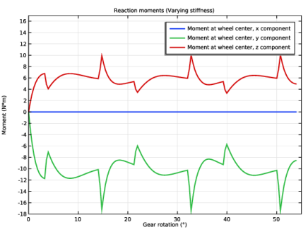
In the Settings window for 1D Plot Group, type Reaction moments (Varying stiffness) in the Label text field.
|
|
3
|
|
1
|
In the Model Builder window, expand the Reaction moments (Varying stiffness) node, then click Global 1.
|
|
2
|
|
1
|
|
2
|
|
3
|
|
4
|
|
5
|
|
1
|
|
2
|
|
3
|
|
4
|
|
5
|
|
1
|
|
2
|
|
1
|
|
2
|
|
3
|
|
4
|
Locate the Physics and Variables Selection section. Select the Modify model configuration for study step check box.
|
|
5
|
In the tree, select Component 1 (comp1)>Multibody Dynamics (mbd)>Hinge Joint: Fixed-Gear 1>Prescribed Motion 1, Component 1 (comp1)>Multibody Dynamics (mbd)>Hinge Joint: Fixed-Gear 2, Component 1 (comp1)>Multibody Dynamics (mbd)>Gear Pair: Constant Stiffness, Component 1 (comp1)>Multibody Dynamics (mbd)>Gear Pair: Varying Stiffness, and Component 1 (comp1)>Multibody Dynamics (mbd)>Gear Pair: Transmission Error.
|
|
6
|
Click
|
|
7
|
|
1
|
|
2
|
|
1
|
|
2
|
|
3
|
|
4
|
|
5
|
|
1
|
|
2
|
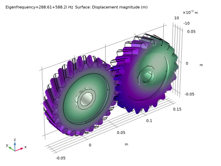
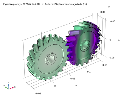
In the Settings window for Study, type Study 6: Eigenfrequency (Constant Stiffness) in the Label text field.
|
|
1
|
In the Model Builder window, under Study 6: Eigenfrequency (Constant Stiffness) click Step 1: Eigenfrequency.
|
|
2
|
|
3
|
|
4
|
In the tree, select Component 1 (comp1)>Multibody Dynamics (mbd)>Hinge Joint: Fixed-Gear 1>Prescribed Motion 1, Component 1 (comp1)>Multibody Dynamics (mbd)>Hinge Joint: Fixed-Gear 2, Component 1 (comp1)>Multibody Dynamics (mbd)>Gear Pair: Rigid, Component 1 (comp1)>Multibody Dynamics (mbd)>Gear Pair: Varying Stiffness, and Component 1 (comp1)>Multibody Dynamics (mbd)>Gear Pair: Transmission Error.
|
|
5
|
Click
|
|
6
|
|
1
|
|
2
|
|
3
|
|
4
|
|
5
|
|
6
|
|
7
|