PDF

CO2 Storage in a Geologic Formation
Introduction
This example models the underground carbon dioxide storage in a part of the Johansen formation. The Johansen reservoir is a saline aquifer off the coast of Norway. The model is inspired by one of the problems in the benchmark study as reported in Ref. 1. The simulation runs over a period of 50 years. In the first 25 years CO2 is injected at a constant rate of 15 kg/s. In the subsequent 25 years, the simulation tracks the spreading of the CO2 due to gravity and capillary forces. This model contains information from the Johansen dataset, which is made available here under the Open Database License (ODbL). Data courtesy of the Norwegian Petroleum Directorate (NPD), the University of Bergen (UiB) and SINTEF.
Model Definition
The part of the reservoir included in the simulation measures approximately 9600 m by 8900 m, with a thickness varying between approximately 90 and 140 m. The geometry, porosity and permeability data are taken from the Johansen dataset (see Ref. 2). The used part of the Johansen formation is shown in Figure 1, with a plot of the porosity distribution. The permeability distribution is shown in Figure 2. The injection well is located at x = 5440 m and y = 3300 m. The total simulation period is 50 years. The CO2 is injected for the first 25 years at a constant rate of 15 kg/s.
The initial conditions for the simulation are a brine filled reservoir at a hydrostatic pressure distribution (hydraulic head of 0 m). The pressure boundary conditions are a hydraulic head of 0 m at the sides, and no flow at the top and bottom boundaries. CO2 saturation is 0 at the side boundaries. The (time constant) geothermal gradient is taken to be 0.030 K/m with a temperature of 100°C at a depth of 3000 m.
The pressure and temperature dependent density and viscosity of the supercritical CO2 are computed using the thermodynamics functionality in COMSOL, using the Peng– Robinson equation of state and the Brokaw model with high pressure correction for the viscosity. The temperature dependent viscosity for the brine is taken to be the viscosity of the Water material from COMSOL Multiphysics’ material library. The pressure and temperature dependent density of the brine is approximated using a thermal expansion coefficient of 6·10-4 1/K, a compressibility of 4·10-10 1/Pa, and a reference density of 1040 kg/m3 at 1·105 Pa and 360 K. Dissolution of CO2 into the brine is not taken into account in this model.
Figure 1: The porosity in the of the part of the Johansen formation that is used for the simulation.
The relative permeabilities and capillary pressure are assumed to be given by the Brooks and Corey capillary pressure model, with the brine being the wetting phase, and with parameters as listed in Table 1.
104 Pa
Figure 2: The permeability in the of the part of the Johansen formation that is used for the simulation.
Results and Discussion
As CO2 is injected, it will start to spread around the well, and it will rise to the top boundary of the formation as the injected CO2 is lighter than the brine, see for example Figure 3 where the CO2 saturation is plotted at the end of the injection phase. During the injection phase, the CO2 plume spreads more or less in all directions, as can been seen in the bottom two plots in Figure 4. Once the injection stops, the CO2 plume spreads further and it also starts to move to the right and up, as seen from the top in Figure 4, against the slope of the top boundary of the formation, due to gravity. It is to be expected that the CO2 plume will eventually reach the right and top boundaries (again as seen from the top) of the simulation domain if the simulation would have been over a longer time period. The results for the spreading of the CO2 plume fit well within the range of the simulation results reported in Ref. 1.
Figure 3: The CO2 saturation after 25 years of injection.
Figure 4: Top view of the formation showing the CO2 saturation after 12.5 years (bottom left), after 25 years (bottom right,) after 37.5 years (top left), and after 50 years (top right).
References
1. H. Class and others, “A Benchmark Study on problems related to CO2 Storage in Geologic Formations,” Comput. Geosci., vol. 13, no. 4, pp. 409–434, 2009.
2. Available at: https://www.sintef.no/projectweb/matmora/downloads/johansen/. The Johansen dataset is made available under the Open Database License: http://opendatacommons.org/licenses/odbl/1.0/. Any rights in individual contents of the database are licensed under the Database Contents License: http://opendatacommons.org/licenses/dbcl/1.0/.
Application Library path: Liquid_and_Gas_Properties_Module/Tutorials/carbon_dioxide_storage
Modeling Instructions
From the File menu, choose New.
New
In the New window, click  Model Wizard.
Model Wizard
1
In the Model Wizard window, click  3D.
2
In the Select Physics tree, select Fluid Flow>Porous Media and Subsurface Flow>Multiphase Flow in Porous Media.
3
Click Add.
4
Click  Study.
5
In the Select Study tree, select General Studies>Time Dependent.
6
Global Definitions
The following instructions import parameter values from a file and use the thermodynamics functionality to set up a material with the necessary materials properties for the subcritical carbon dioxide that is injected in the formation.
Parameters 1
1
In the Model Builder window, under Global Definitions click Parameters 1.
2
In the Settings window for Parameters, locate the Parameters section.
3
Click  Load from File.
4
5
In the Physics toolbar, click  Thermodynamics and choose Thermodynamic System.
Select System
1
Go to the Select System window.
2
Click Next in the window toolbar.
Select Species
1
Go to the Select Species window.
2
In the Species list, select carbon dioxide (124-38-9, CO2).
3
Click  Add Selected.
4
Click Next in the window toolbar.
Select Thermodynamic Model
1
Go to the Select Thermodynamic Model window.
2
From the Gas phase model list, choose Peng-Robinson.
3
Select the Advanced options check box.
4
5
Click Finish in the window toolbar.
Global Definitions
Gas System 1 (pp1)
In the Model Builder window, under Global Definitions>Thermodynamics right-click Gas System 1 (pp1) and choose Generate Material.
Select Phase
1
Go to the Select Phase window.
2
Click Next in the window toolbar.
Select Species
1
Go to the Select Species window.
2
Click Next in the window toolbar.
Select Properties
1
Go to the Select Properties window.
2
Click Next in the window toolbar.
Define Material
1
Go to the Define Material window.
2
From the Function type list, choose Interpolation.
3
From the Maximum number of interpolation points list, choose Fine (2500).
4
In row Temperature, set High to 400.
5
In row Temperature, set Number of points to 30.
6
In row Pressure, set Low to 1e5.
7
In row Pressure, set High to 4e7.
8
In row Pressure, set Number of points to 80.
9
Click Finish in the window toolbar.
Definitions
The following instructions define the geothermal temperature distribution and import the porosity and permeability distributions in the formation and set up interpolation functions for use in the simulation.
Variables 1
1
In the Model Builder window, under Component 1 (comp1) right-click Definitions and choose Variables.
2
In the Settings window for Variables, locate the Variables section.
3
Interpolation 1 (int1)
1
In the Home toolbar, click  Functions and choose Local>Interpolation.
2
In the Settings window for Interpolation, locate the Definition section.
3
From the Data source list, choose File.
4
Click  Browse.
5
6
Find the Functions subsection. In the table, enter the following settings:
7
Locate the Units section. In the Function table, enter the following settings:
8
In the Argument table, enter the following settings:
9
Locate the Definition section. Click  Import.
10
Select the Use spatial coordinates as arguments check box.
11
From the Frame list, choose Mesh.
12
Select the Reinterpolate interpolation data on computational mesh check box. This makes sure that the interpolation function is evaluated using cached values at Lagrange points on the computational mesh, resulting in a much more efficient evaluation during the computation.
Interpolation 2 (int2)
1
In the Home toolbar, click  Functions and choose Local>Interpolation.
2
In the Settings window for Interpolation, locate the Definition section.
3
From the Data source list, choose File.
4
Click  Browse.
5
6
Find the Functions subsection. In the table, enter the following settings:
7
Locate the Units section. In the Function table, enter the following settings:
8
In the Argument table, enter the following settings:
9
Locate the Definition section. Click  Import.
10
Select the Use spatial coordinates as arguments check box.
11
From the Frame list, choose Mesh.
12
Select the Reinterpolate interpolation data on computational mesh check box.
Analytic 1 (an1)
1
In the Home toolbar, click  Functions and choose Local>Analytic.
2
In the Settings window for Analytic, type density_brine in the Function name text field.
3
Locate the Definition section. In the Expression text field, type rho0-rho0*alpha*(T-T0)+rho0*beta*(p-p0).
4
In the Arguments text field, type T, p.
5
Locate the Units section. In the Function text field, type kg/m^3.
6
The following instructions add a rectangle function. It will be used at the injection well to gradually ramp up the carbon dioxide injection rate over a period of 0.1 year and to switch it off after 25 years.
Rectangle 1 (rect1)
1
In the Home toolbar, click  Functions and choose Local>Rectangle.
2
In the Settings window for Rectangle, locate the Parameters section.
3
In the Lower limit text field, type 0.05.
4
In the Upper limit text field, type 25.
Geometry 1
The following instructions import the geometry of the Johansen formation and create an edge at the position of the injection well. Around the well a block is created for meshing purposes.
Import 1 (imp1)
1
In the Home toolbar, click  Import.
2
In the Settings window for Import, locate the Import section.
3
Click  Browse.
4
5
Click  Import.
Line Segment 1 (ls1)
1
In the Geometry toolbar, click  More Primitives and choose Line Segment.
2
In the Settings window for Line Segment, locate the Starting Point section.
3
From the Specify list, choose Coordinates.
4
In the x text field, type x_well.
5
In the y text field, type y_well.
6
In the z text field, type -3200.
7
Locate the Endpoint section. From the Specify list, choose Coordinates.
8
In the x text field, type x_well.
9
In the y text field, type y_well.
10
In the z text field, type -2500.
Block 1 (blk1)
1
In the Geometry toolbar, click  Block.
2
In the Settings window for Block, locate the Size and Shape section.
3
In the Width text field, type 100.
4
In the Depth text field, type 100.
5
In the Height text field, type 500.
6
Locate the Position section. In the x text field, type x_well-50.
7
In the y text field, type y_well-50.
8
In the z text field, type -3200.
Partition Objects 1 (par1)
1
In the Geometry toolbar, click  Booleans and Partitions and choose Partition Objects.
2
Select the objects blk1 and ls1 only.
3
In the Settings window for Partition Objects, locate the Partition Objects section.
4
Find the Tool objects subsection. Click to select the  Activate Selection toggle button.
5
6
Select the Keep tool objects check box.
Delete Entities 1 (del1)
1
In the Model Builder window, right-click Geometry 1 and choose Delete Entities.
2
In the Settings window for Delete Entities, locate the Entities or Objects to Delete section.
3
From the Geometric entity level list, choose Domain.
4
On the object par1(1), select Domains 1 and 3 only.
Delete Entities 2 (del2)
1
Right-click Geometry 1 and choose Delete Entities.
2
In the Settings window for Delete Entities, locate the Entities or Objects to Delete section.
3
From the Geometric entity level list, choose Edge.
4
On the object par1(2), select Edges 1 and 3 only.
Partition Edges 1 (pare1)
1
In the Geometry toolbar, click  Booleans and Partitions and choose Partition Edges.
2
On the object del2, select Edge 1 only.
3
In the Settings window for Partition Edges, locate the Positions section.
4
Delete Entities 3 (del3)
1
Right-click Geometry 1 and choose Delete Entities.
2
In the Settings window for Delete Entities, locate the Entities or Objects to Delete section.
3
From the Geometric entity level list, choose Edge.
4
On the object pare1, select Edges 1 and 3 only.
5
Click  Build All Objects.
Add Material
1
In the Home toolbar, click  Add Material to open the Add Material window.
2
Go to the Add Material window.
3
In the tree, select Built-in>Water, liquid.
4
Click Add to Component in the window toolbar.
5
In the Home toolbar, click  Add Material to close the Add Material window.
Phase Transport in Porous Media (phtr)
1
Click the  Show More Options button in the Model Builder toolbar.
2
In the Show More Options dialog box, in the tree, select the check box for the node Physics>Advanced Physics Options.
3
4
In the Model Builder window, under Component 1 (comp1) click Phase Transport in Porous Media (phtr).
5
In the Settings window for Phase Transport in Porous Media, locate the Gravity Effects section.
6
Select the Include gravity check box.
7
Click to expand the Quadrature Settings section. Clear the Use automatic quadrature settings check box.
8
In the Integration order text field, type 4. This increases the default integration order to guaranty a more accurate evaluation of the nonlinear coefficients in the equations.
Phase and Porous Media Transport Properties 1
1
In the Model Builder window, under Component 1 (comp1)>Phase Transport in Porous Media (phtr) click Phase and Porous Media Transport Properties 1.
2
In the Settings window for Phase and Porous Media Transport Properties, locate the Model Input section.
3
From the T list, choose User defined. In the associated text field, type Temp.
4
Locate the Capillary Pressure section. From the Capillary pressure model list, choose Brooks and Corey.
5
In the pec text field, type pc_e.
6
In the λp text field, type lambda.
7
Locate the Phase 1 Properties section. From the Fluid s1 list, choose Water, liquid (mat1).
8
Locate the Phase 2 Properties section. From the Fluid s2 list, choose Gas: carbon dioxide(1) 1 (pp1mat1).
9
Locate the Phase 1 Properties section. From the ρs1 list, choose User defined. In the associated text field, type density_brine(Temp,dl.pA).
10
In the srs1 text field, type s0_b.
Volume Fraction 1
1
In the Physics toolbar, click  Boundaries and choose Volume Fraction.
2
3
In the Settings window for Volume Fraction, locate the Boundary Selection section.
4
Click  Create Selection.
5
In the Create Selection dialog box, type Sides in the Selection name text field.
6
7
In the Settings window for Volume Fraction, locate the Volume Fraction section.
8
Select the Phase s2 check box.
Darcy’s Law (dl)
1
In the Model Builder window, under Component 1 (comp1) click Darcy’s Law (dl).
2
In the Settings window for Darcy’s Law, locate the Gravity Effects section.
3
Select the Include gravity check box.
4
Click to expand the Discretization section. From the Pressure list, choose Linear. Switching to a lower element order reduces the number of degrees of freedom to make the simulation more computationally efficient. Since the used mesh is quite fine, this will not reduce the accuracy significantly.
Porous Matrix 1
1
In the Model Builder window, under Component 1 (comp1)>Darcy’s Law (dl)>Porous Medium 1 click Porous Matrix 1.
2
In the Settings window for Porous Matrix, locate the Matrix Properties section.
3
From the εp list, choose User defined. In the associated text field, type porosity.
4
From the κ list, choose User defined. In the associated text field, type permeability.
Initial Values 1
1
In the Model Builder window, under Component 1 (comp1)>Darcy’s Law (dl) click Initial Values 1.
2
In the Settings window for Initial Values, locate the Initial Values section.
3
Click the Hydraulic head button.
Hydraulic Head 1
1
In the Physics toolbar, click  Boundaries and choose Hydraulic Head.
2
In the Settings window for Hydraulic Head, locate the Boundary Selection section.
3
From the Selection list, choose Sides.
Multiphysics
Well 1 (wellmpe1)
1
In the Physics toolbar, click  Multiphysics Couplings and choose Edge>Well.
2
3
In the Settings window for Well, locate the Well section.
4
In the M0 text field, type r_injection*rect1(t/1[a]).
5
Locate the Phase 2 section. In the M0,s2 text field, type r_injection*rect1(t/1[a]).
Mesh 1
Free Triangular 1
In the Mesh toolbar, click  Boundary and choose Free Triangular.
Size
1
In the Model Builder window, click Size.
2
In the Settings window for Size, locate the Element Size section.
3
From the Calibrate for list, choose Fluid dynamics.
4
From the Predefined list, choose Finer.
5
Click the Custom button.
6
Locate the Element Size Parameters section. In the Maximum element size text field, type 120.
Free Triangular 1
1
In the Model Builder window, click Free Triangular 1.
2
Swept 1
1
In the Mesh toolbar, click  Swept.
2
In the Settings window for Swept, locate the Domain Selection section.
3
From the Geometric entity level list, choose Domain.
4
Distribution 1
1
Right-click Swept 1 and choose Distribution.
2
In the Settings window for Distribution, locate the Distribution section.
3
In the Number of elements text field, type 9.
Edge 1
1
In the Mesh toolbar, click  Boundary and choose Edge.
2
Distribution 1
Right-click Edge 1 and choose Distribution.
Free Tetrahedral 1
1
In the Mesh toolbar, click  Free Tetrahedral.
2
In the Settings window for Free Tetrahedral, click to expand the Scale Geometry section.
3
In the z-direction scale text field, type 10.
Size 1
1
Right-click Free Tetrahedral 1 and choose Size.
2
In the Settings window for Size, locate the Geometric Entity Selection section.
3
From the Geometric entity level list, choose Domain.
4
5
Locate the Element Size section. From the Predefined list, choose Finer.
6
Click  Build All.
Study 1
Step 1: Time Dependent
1
In the Model Builder window, under Study 1 click Step 1: Time Dependent.
2
In the Settings window for Time Dependent, locate the Study Settings section.
3
From the Time unit list, choose a.
4
In the Output times text field, type range(0,2.5,50).
5
From the Tolerance list, choose User controlled.
6
In the Relative tolerance text field, type 0.001.
Solution 1 (sol1)
1
In the Study toolbar, click  Show Default Solver.
2
In the Model Builder window, expand the Solution 1 (sol1) node, then click Dependent Variables 1.
3
In the Settings window for Dependent Variables, locate the Scaling section.
4
From the Method list, choose Initial value based.
5
In the Model Builder window, expand the Study 1>Solver Configurations>Solution 1 (sol1)>Time-Dependent Solver 1 node, then click Fully Coupled 1.
6
In the Settings window for Fully Coupled, click to expand the Method and Termination section.
7
From the Jacobian update list, choose Minimal.
8
In the Tolerance factor text field, type 0.5.
9
In the Study toolbar, click  Compute.
Definitions
Since the geometry of the formation is thin in the vertical direction, it can be difficult to get a good impression of the distribution of the results in the z direction in plots. The following instructions change the view settings such that the plots are scaled in the vertical direction to get a better impression of the results.
Camera
1
In the Model Builder window, expand the Component 1 (comp1)>Definitions>View 1 node, then click Camera.
2
In the Settings window for Camera, locate the Camera section.
3
From the View scale list, choose Manual.
4
In the z scale text field, type 5.
Create a new plot for the porosity.
Results
Porosity
1
In the Home toolbar, click  Add Plot Group and choose 3D Plot Group.
2
In the Settings window for 3D Plot Group, type Porosity in the Label text field.
Contour 1
1
Right-click Porosity and choose Contour.
2
In the Settings window for Contour, locate the Expression section.
3
In the Expression text field, type porosity.
4
Locate the Levels section. In the Total levels text field, type 10.
5
Locate the Coloring and Style section. From the Contour type list, choose Filled.
Porosity
1
In the Model Builder window, click Porosity.
2
In the Settings window for 3D Plot Group, click to expand the Title section.
3
From the Title type list, choose Manual.
4
In the Title text area, type Porosity.
5
Clear the Parameter indicator text field.
6
In the Porosity toolbar, click  Plot.
7
Click the  Zoom Extents button in the Graphics toolbar.
The previous instructions created the plot of the porosity as shown in Figure 1. Reproduce the plot in Figure 2 by replacing the expression in the Expression text field by permeability.
The following instructions create the plots in Figure 3 and Figure 4.
Cut Plane 1
1
In the Model Builder window, expand the Results>Datasets node.
2
Right-click Results>Datasets and choose Cut Plane.
3
In the Settings window for Cut Plane, locate the Plane Data section.
4
In the x-coordinate text field, type 6000.
5
Select the Additional parallel planes check box.
6
In the Distances text field, type range(-6000,500,9000).
CO2 Saturation
1
In the Results toolbar, click  3D Plot Group.
2
In the Settings window for 3D Plot Group, type CO2 Saturation in the Label text field.
3
Locate the Data section. From the Time (a) list, choose 25.
Contour 1
1
Right-click CO2 Saturation and choose Contour.
2
In the Settings window for Contour, locate the Data section.
3
From the Dataset list, choose Cut Plane 1.
4
From the Solution parameters list, choose From parent.
5
Locate the Expression section. In the Expression text field, type s2.
6
Locate the Levels section. In the Total levels text field, type 5.
7
Locate the Coloring and Style section. From the Contour type list, choose Filled.
8
In the Graphics window toolbar, clicknext to  Scene Light, then choose Ambient Occlusion.
9
In the CO2 Saturation toolbar, click  Plot.
Surface 1
1
In the Results toolbar, click  More Datasets and choose Surface.
2
2D Plot Group 7
In the Results toolbar, click  2D Plot Group.
Surface 1
1
Right-click 2D Plot Group 7 and choose Surface.
2
In the Settings window for Surface, locate the Expression section.
3
In the Expression text field, type s2.
CO2 Saturation, Top View
1
In the Model Builder window, under Results click 2D Plot Group 7.
2
In the Settings window for 2D Plot Group, type CO2 Saturation, Top View in the Label text field.
3
Locate the Data section. From the Dataset list, choose Surface 1.
4
From the Time (a) list, choose 12.5.
5
Click to expand the Title section. From the Title type list, choose Manual.
6
Clear the Parameter indicator text field.
7
In the Title text area, type CO2 saturation.
8
Click to expand the Plot Array section. Select the Enable check box.
9
From the Array shape list, choose Square.
Surface 2
1
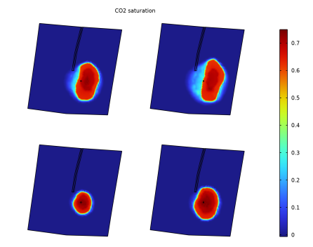
In the Model Builder window, under Results>CO2 Saturation, Top View right-click Surface 1 and choose Duplicate.
2
In the Settings window for Surface, locate the Data section.
3
From the Dataset list, choose Surface 1.
4
From the Time (a) list, choose 25.
5
Click to expand the Inherit Style section. From the Plot list, choose Surface 1.
Surface 3
1
Right-click Surface 2 and choose Duplicate.
2
In the Settings window for Surface, locate the Data section.
3
From the Time (a) list, choose 37.5.
Surface 4
1
Right-click Surface 3 and choose Duplicate.
2
In the Settings window for Surface, click  Plot Last.
3
Click the  Show Grid button in the Graphics toolbar.
4
In the CO2 Saturation, Top View toolbar, click  Plot.