PDF

Spacecraft Thermal Analysis
Introduction
This model demonstrates how to compute satellite temperature over multiple orbit periods by coupling Orbital Thermal Loads to Heat Transfer in Solids. The direct solar, albedo, and Earth infrared thermal loads are computed over a single orbit, and are periodically repeated over multiple orbits.
A 1U CubeSat in a circular 400 km altitude orbit is rotating about its nadir-pointing axis. A geometric model of the satellite considers the frame, boards, sensor, interior instruments, and solar cells.
The solar cells are modeled as having zero thickness to reduce the geometric complexity, and are modeled via a boundary condition that considers the thickness and material properties. The conversion of the incident light into electricity is modeled via an additional heat load that accounts for the nonthermal absorption.
The instruments within the satellite generate heat, and one of the instruments switches to a higher power mode during part of the eclipse period. The objective of the simulation is to predict the temperature over time.
Model Definition
Figure 1: Cutout view of the satellite geometry.
Figure 1 shows the geometry used to model the satellite. An aluminum frame has circuit boards mounted on the sides and within. The outside boards have solar cells on the surface, but these are not explicitly represented in the geometry. Instead, they will be modeled via a boundary condition. The board on the inside has instruments mounted on both sides, as well as a sensor that protrudes through the board on the top. Although the geometry here is simplified, and contains less components than a real satellite, the overall modeling workflow is similar regardless of the complexity of the geometry.
The model uses a combination of the Heat Transfer in Solids interface, which computes the temperature within the solid structure, and the Orbital Thermal Loads, which computes the environmental radiative loads and the heat exchange between surfaces. The environmental loads are computed based upon the orbital parameters as well as the satellite orientation. This is demonstrated in the example Orbit Calculation.
There are three sets of radiative boundary conditions used. For the surfaces facing the exterior of the satellite, the emissivities are specified via the two-band solar and ambient model. The solar cells have an emissivity in the solar band of 0.99 and 0.95 in the ambient band. The solar cells absorb light very well, but convert a fraction of the incident light in the solar band into electrical energy rather than heat, this is accounted for via a boundary condition in the Heat Transfer in Solids interface. The remaining exterior surfaces have an emissivity of 0.2 in the solar band, and 0.85 in the ambient. This represents a surface coating that reflects well in the solar band, and emits well in the ambient band, to keep the satellite as cool as possible. For radiative heat exchange within the interior of the satellite, a constant emissivity of 0.8 is used for all surfaces to model radiative heat exchange within the interior.
The two instruments mounted on the board within the satellite are modeled as solid copper, with a heat load uniformly distributed over the volume. The smaller instrument dissipates 1 W continuously, and the larger dissipates 0.5 W, but during the eclipse switches to a higher-power mode, dissipating 5 W. The higher-power mode begins 20 minutes after entering eclipse, and lasts for 15 minutes. The switching of magnitude is controlled via the Events interface.
The solar cells are modeled via the Thin Layer boundary condition which accounts for heat transfer through the thickness as well as along the surface. To account for the conversion of light into electric energy rather than thermal energy, a heat load of negative magnitude is applied, which is equivalent to reducing the absorbed environmental heat load in the solar band at those surfaces.
The instruments and sensors are mounted onto the interior board, and this mounting is approximated via a surface resistance specified in a Thermal Contact boundary condition. This introduces a jump in temperature across the boundary. At all other mating boundaries the temperature field is continuous between parts.
The solution procedure involves two study steps. In the first step, the environmental loads are computed over a single orbit, since it is assumed that these loads will not change significantly over several orbits. In the second step, the loads are periodically repeated over four orbits.
Results and Discussion
Figure 2 displays the temperature of the satellite after 4 orbit periods.
Figure 2: Temperature field on the sensor, instruments, and interior board.
Figure 3 shows the evolution of the maximum and minimum temperature over time. It shows that it takes several orbits for the solution to become periodic.
Figure 3: Maximum and minimum temperature on the satellite boundaries over time. The red line indicates when the satellite is exposed to the Sun.
Application Library path: Heat_Transfer_Module/Orbital_Thermal_Loads/spacecraft_thermal_analysis
Model Instructions
From the File menu, choose New.
New
In the New window, click  Model Wizard.
Model Wizard
1
In the Model Wizard window, click  3D.
2
In the Select Physics tree, select Heat Transfer>Radiation>Heat Transfer with Orbital Thermal Loads.
3
Click Add.
4
Click  Study.
5
In the Select Study tree, select Preset Studies for Selected Physics Interfaces>Orbital Thermal Loads>Orbital Temperature.
6
Global Definitions
Parameters 1
1
In the Model Builder window, under Global Definitions click Parameters 1.
2
In the Settings window for Parameters, locate the Parameters section.
3
Geometry 1
Block 1 (blk1)
1
In the Model Builder window, expand the Component 1 (comp1)>Geometry 1 node.
2
Right-click Geometry 1 and choose Block.
3
In the Settings window for Block, locate the Size and Shape section.
4
In the Width text field, type 10[cm].
5
In the Depth text field, type 10[cm].
6
In the Height text field, type 10[cm].
7
Locate the Position section. From the Base list, choose Center.
Block 2 (blk2)
1
In the Geometry toolbar, click  Block.
2
In the Settings window for Block, locate the Size and Shape section.
3
In the Width text field, type 9[cm].
4
In the Depth text field, type 9[cm].
5
In the Height text field, type 9[cm].
6
Locate the Position section. From the Base list, choose Center.
Difference 1 (dif1)
1
In the Geometry toolbar, click  Booleans and Partitions and choose Difference.
2
3
In the Settings window for Difference, locate the Difference section.
4
Find the Objects to subtract subsection. Click to select the  Activate Selection toggle button.
5
Block 3 (blk3)
1
In the Geometry toolbar, click  Block.
2
In the Settings window for Block, locate the Size and Shape section.
3
In the Width text field, type 9[cm].
4
In the Depth text field, type 9[cm].
5
In the Height text field, type 5[mm].
6
Locate the Position section. From the Base list, choose Center.
7
In the z text field, type 4.75[cm].
Mirror 1 (mir1)
1
In the Geometry toolbar, click  Transforms and choose Mirror.
2
3
In the Settings window for Mirror, locate the Input section.
4
Select the Keep input objects check box.
Rotate 1 (rot1)
1
In the Geometry toolbar, click  Transforms and choose Rotate.
2
Select the objects blk3 and mir1 only.
3
In the Settings window for Rotate, locate the Input section.
4
Select the Keep input objects check box.
5
Locate the Rotation section. From the Axis type list, choose y-axis.
6
In the Angle text field, type 90.
Rotate 2 (rot2)
1
In the Geometry toolbar, click  Transforms and choose Rotate.
2
Select the objects rot1(1) and rot1(2) only.
3
In the Settings window for Rotate, locate the Input section.
4
Select the Keep input objects check box.
5
Locate the Rotation section. In the Angle text field, type 90.
Difference 2 (dif2)
1
In the Geometry toolbar, click  Booleans and Partitions and choose Difference.
2
3
In the Settings window for Difference, locate the Difference section.
4
Find the Objects to subtract subsection. Click to select the  Activate Selection toggle button.
5
Select the objects blk3, mir1, rot1(1), rot1(2), rot2(1), and rot2(2) only.
6
Select the Keep objects to subtract check box.
Block 4 (blk4)
1
In the Geometry toolbar, click  Block.
2
In the Settings window for Block, locate the Size and Shape section.
3
In the Width text field, type 9[cm].
4
In the Depth text field, type 9[cm].
5
In the Height text field, type 5[mm].
6
Locate the Position section. From the Base list, choose Center.
Block 5 (blk5)
1
In the Geometry toolbar, click  Block.
2
In the Settings window for Block, locate the Size and Shape section.
3
In the Width text field, type 3[cm].
4
In the Depth text field, type 6[cm].
5
In the Height text field, type 2[cm].
6
Locate the Position section. In the x text field, type -3[cm].
7
In the y text field, type -3.5[cm].
8
In the z text field, type -2.25[cm].
Block 6 (blk6)
1
In the Geometry toolbar, click  Block.
2
In the Settings window for Block, locate the Size and Shape section.
3
In the Width text field, type 1.5[cm].
4
In the Depth text field, type 2[cm].
5
In the Height text field, type 0.75[cm].
6
Locate the Position section. In the x text field, type 2.5[cm].
7
In the y text field, type -4[cm].
8
In the z text field, type 0.25[cm].
Cylinder 1 (cyl1)
1
In the Geometry toolbar, click  Cylinder.
2
In the Settings window for Cylinder, locate the Size and Shape section.
3
In the Radius text field, type 2[cm].
4
In the Height text field, type 6.5[cm].
5
Locate the Position section. In the z text field, type 2.5[mm].
Difference 3 (dif3)
1
In the Geometry toolbar, click  Booleans and Partitions and choose Difference.
2
3
In the Settings window for Difference, locate the Difference section.
4
Find the Objects to subtract subsection. Click to select the  Activate Selection toggle button.
5
6
Select the Keep objects to subtract check box.
Cylinder 2 (cyl2)
1
In the Geometry toolbar, click  Cylinder.
2
In the Settings window for Cylinder, locate the Size and Shape section.
3
In the Radius text field, type 1.8[cm].
4
In the Height text field, type 6.5[cm].
5
Locate the Position section. In the z text field, type 2[cm].
Difference 4 (dif4)
1
In the Geometry toolbar, click  Booleans and Partitions and choose Difference.
2
3
In the Settings window for Difference, locate the Difference section.
4
Find the Objects to subtract subsection. Click to select the  Activate Selection toggle button.
5
Form Union (fin)
1
In the Geometry toolbar, click  Build All.
Now that the geometry is created, define selections to reuse for the material and feature selections.
Definitions
Define a selection consisting of all exterior boundaries of all domains. Radiation from all of these faces will be considered.
All Radiative Boundaries
1
In the Model Builder window, expand the Component 1 (comp1)>Definitions node.
2
Right-click Definitions and choose Selections>Explicit.
3
In the Settings window for Explicit, type All Radiative Boundaries in the Label text field.
4
Locate the Input Entities section. Select the All domains check box.
5
Locate the Output Entities section. From the Output entities list, choose Adjacent boundaries.
Define a selection consisting of all boundaries that are facing the exterior void. These are the boundaries that can be exposed to environmental loads.
Space-Facing Boundaries
1
In the Definitions toolbar, click  Explicit.
2
In the Settings window for Explicit, locate the Input Entities section.
3
Click  Paste Selection.
4
In the Paste Selection dialog box, type 0 in the Selection text field.
5
6
In the Settings window for Explicit, locate the Output Entities section.
7
From the Output entities list, choose Adjacent boundaries.
8
In the Label text field, type Space-Facing Boundaries.
Solar Cells
1
In the Definitions toolbar, click  Explicit.
2
In the Settings window for Explicit, type Solar Cells in the Label text field.
3
Locate the Input Entities section. From the Geometric entity level list, choose Boundary.
4
Click  Paste Selection.
5
In the Paste Selection dialog box, type 5 12 39 83 in the Selection text field.
6
Add operators to evaluate maximum and minimum temperature over the model.
Maximum on All Domains
1
In the Definitions toolbar, click  Nonlocal Couplings and choose Maximum.
2
In the Settings window for Maximum, type Maximum on All Domains in the Label text field.
3
Locate the Source Selection section. From the Selection list, choose All domains.
Minimum on All Domains
1
In the Definitions toolbar, click  Nonlocal Couplings and choose Minimum.
2
In the Settings window for Minimum, type Minimum on All Domains in the Label text field.
3
Locate the Source Selection section. From the Selection list, choose All domains.
Add Material
1
In the Home toolbar, click  Add Material to open the Add Material window.
2
Go to the Add Material window.
3
In the tree, select Built-in>Aluminum.
4
Click Add to Component in the window toolbar.
5
In the tree, select Built-in>Copper.
6
Click Add to Component in the window toolbar.
7
In the tree, select Built-in>FR4 (Circuit Board).
8
Click Add to Component in the window toolbar.
9
In the tree, select Built-in>Silicon.
10
Click Add to Component in the window toolbar.
11
In the tree, select Built-in>Titanium beta-21S.
12
Click Add to Component in the window toolbar.
Materials
Copper (mat2)
1
In the Model Builder window, under Component 1 (comp1)>Materials click Copper (mat2).
2
In the Settings window for Material, locate the Geometric Entity Selection section.
3
Click  Paste Selection.
4
In the Paste Selection dialog box, type 8 10 in the Selection text field.
5
FR4 (Circuit Board) (mat3)
1
In the Model Builder window, click FR4 (Circuit Board) (mat3).
2
In the Settings window for Material, locate the Geometric Entity Selection section.
3
Click  Paste Selection.
4
In the Paste Selection dialog box, type 2-7, 11 in the Selection text field.
5
Silicon (mat4)
1
In the Model Builder window, click Silicon (mat4).
2
In the Settings window for Material, locate the Geometric Entity Selection section.
3
From the Geometric entity level list, choose Boundary.
4
From the Selection list, choose Solar Cells.
Titanium beta-21S (mat5)
1
In the Model Builder window, click Titanium beta-21S (mat5).
2
In the Settings window for Material, locate the Geometric Entity Selection section.
3
Click  Paste Selection.
4
In the Paste Selection dialog box, type 9 in the Selection text field.
5
The larger instrument dissipates 0.5 W, but it switches to a higher-power mode for 15 minutes during the eclipse, dissipating 5 W.
Heat Transfer in Solids (ht)
Heat Source 1
1
In the Model Builder window, under Component 1 (comp1) right-click Heat Transfer in Solids (ht) and choose Heat Source.
2
In the Settings window for Heat Source, locate the Domain Selection section.
3
Click  Paste Selection.
4
In the Paste Selection dialog box, type 8 in the Selection text field.
5
HS1 is an indicator controlled by the Events interface. It’s enabled 20 minutes after entering eclipse, and lasts for 15 minutes.
6
In the Settings window for Heat Source, locate the Heat Source section.
7
From the Heat source list, choose Heat rate.
8
In the P0 text field, type 0.5[W]+4.5[W]*HS1.
Add a heat source on the smaller instrument that dissipates 1 W continuously.
Heat Source 2
1
In the Physics toolbar, click  Domains and choose Heat Source.
2
3
In the Settings window for Heat Source, locate the Heat Source section.
4
From the Heat source list, choose Heat rate.
5
In the P0 text field, type 1.
The solar cells are modeled via the Thin Layer boundary condition, of type General, which accounts for heat transfer through the thickness as well as along the surface.
Thin Layer 1
1
In the Physics toolbar, click  Boundaries and choose Thin Layer.
2
In the Settings window for Thin Layer, locate the Boundary Selection section.
3
From the Selection list, choose Solar Cells.
4
Locate the Layer Model section. From the Layer type list, choose General.
Materials
Silicon (mat4)
1
In the Model Builder window, expand the Component 1 (comp1)>Materials>Silicon (mat4) node, then click Silicon (mat4).
2
In the Settings window for Material, locate the Material Contents section.
3
4
Locate the Orientation and Position section. From the Position list, choose Bottom side on boundary.
The instruments and sensors are mounted onto the interior board, and this mounting is approximated via a surface resistance specified in a Thermal Contact boundary condition. This introduces a jump in temperature across the boundary.
Heat Transfer in Solids (ht)
Thermal Contact 1
1
In the Physics toolbar, click  Boundaries and choose Thermal Contact.
2
3
In the Settings window for Thermal Contact, locate the Thermal Contact section.
4
From the Contact model list, choose Equivalent thin resistive layer.
5
In the Req text field, type 0.01.
To account for the conversion of light into electric energy rather than thermal energy. The corresponding energy loss is modeled using a heat flux condition on the solar cells boundaries.
Heat Flux 1
1
In the Physics toolbar, click  Boundaries and choose Heat Flux.
2
In the Settings window for Heat Flux, locate the Boundary Selection section.
3
From the Selection list, choose Solar Cells.
4
Locate the Heat Flux section. In the q0 text field, type -otl.Grad_band1*Efficiency.
Orbital Thermal Loads (otl)
1
In the Model Builder window, under Component 1 (comp1) click Orbital Thermal Loads (otl).
2
In the Settings window for Orbital Thermal Loads, locate the Boundary Selection section.
3
From the Selection list, choose All Radiative Boundaries.
Sun Properties 1
By default, the Sun vector and solar flux are set to correspond to the winter solstice.
Planet Properties 1
1
In the Model Builder window, click Planet Properties 1.
2
In the Settings window for Planet Properties, locate the Planet Properties section.
3
Find the Planet initial position subsection. From the Planet longitude at start time list, choose Longitude at subspacecraft point.
The Earth properties are used to define the planet.
4
Locate the Radiative Properties section. From the Albedo list, choose User defined distribution.
The proportion of solar radiation incident onto Earth reflected diffusely back towards the satellite, or albedo, is set to 0.3 everywhere on the planet.
5
In the α0,λ text field, type 0.3.
Earth is relatively warm compared to background deep space and is modeled as a distributed emitter having a uniform flux of 225 W/m^2.
6
From the Planet infrared flux list, choose User defined for each band.
7
Orbital Parameters 1
A circular orbit is defined at 400 km altitude, inclination of 50°, and local time at ascending node set to 15 h.
1
In the Model Builder window, click Orbital Parameters 1.
2
In the Settings window for Orbital Parameters, locate the Orbital Parameters section.
3
From the Orbit type list, choose Circular.
4
In the R text field, type otl.R_planet+400[km].
5
In the i text field, type 50[deg].
6
From the Ascending node list, choose Local time at ascending node.
7
In the tΩ text field, type 15[h].
Spacecraft Orientation 1
The orientation of the satellite is such that the primary direction points towards Earth. The satellite is slowly rotating about its primary axis, so the secondary axis can be any vector that is not parallel to nadir. In this case the default setting, of the +X direction corresponding to the direction of travel, is used.
1
In the Model Builder window, click Spacecraft Orientation 1.
2
In the Settings window for Spacecraft Orientation, locate the Spacecraft Orientation section.
3
Find the Rotations subsection. From the Rotation about primary axis list, choose Angular rate.
4
In the ω text field, type 2*360[deg]/otl.T_orbit.
Generate Events Interface 1
In order to handle the passing of the spacecraft through the eclipse, an Events interface is necessary and should always be added when using the Orbital Thermal Loads physics.
1
In the Model Builder window, click Generate Events Interface 1.
2
In the Settings window for Generate Events Interface, locate the Generate Events Interface section.
3
Click Create New.
Diffuse Surface, Inside
Now, define the radiative properties of the different boundaries.
1
In the Model Builder window, under Component 1 (comp1)>Orbital Thermal Loads (otl) click Diffuse Surface 1.
2
In the Settings window for Diffuse Surface, type Diffuse Surface, Inside in the Label text field.
3
Locate the Surface Emissivity section. From the ε list, choose User defined. In the associated text field, type 0.8.
Diffuse Surface, Outside
1
In the Physics toolbar, click  Boundaries and choose Diffuse Surface.
2
In the Settings window for Diffuse Surface, locate the Boundary Selection section.
3
From the Selection list, choose Space-Facing Boundaries.
4
In the Label text field, type Diffuse Surface, Outside.
5
Locate the Surface Emissivity section. From the ε list, choose User defined for each band.
6
Diffuse Surface, Solar Cells
1
In the Physics toolbar, click  Boundaries and choose Diffuse Surface.
2
In the Settings window for Diffuse Surface, locate the Boundary Selection section.
3
From the Selection list, choose Solar Cells.
4
In the Label text field, type Diffuse Surface, Solar Cells.
5
Locate the Surface Emissivity section. From the ε list, choose User defined for each band.
6
The following features need to be added to control the switching of magnitude of the heat source in the larger instrument when entering the eclipse.
Events 1 (ev)
In the Model Builder window, under Component 1 (comp1) click Events 1 (ev).
Instrument 1, State Variable
1
In the Physics toolbar, click  Global and choose Discrete States.
2
In the Settings window for Discrete States, type Instrument 1, State Variable in the Label text field.
3
Locate the Discrete States section. In the table, enter the following settings:
Instrument 1, Turn On
1
In the Physics toolbar, click  Global and choose Explicit Event.
2
In the Settings window for Explicit Event, type Instrument 1, Turn On in the Label text field.
3
Locate the Event Timings section. In the ti text field, type otl.t_inEclipse+20[min].
4
In the T text field, type otl.T_eclipse.
5
Locate the Reinitialization section. In the table, enter the following settings:
Instrument 1, Turn Off
1
In the Physics toolbar, click  Global and choose Explicit Event.
2
In the Settings window for Explicit Event, type Instrument 1, Turn Off in the Label text field.
3
Locate the Event Timings section. In the ti text field, type otl.t_inEclipse+20[min]+15[min].
4
In the T text field, type otl.T_eclipse.
5
Locate the Reinitialization section. In the table, enter the following settings:
The solution procedure involves two study steps. In the first step, the environmental loads are computed over a single orbit, since it is assumed that these loads will not change significantly over several orbits. In the second step, the loads are periodically repeated over four orbits.
Study 1
Step 1: Orbit Thermal Loads
1
In the Model Builder window, under Study 1 click Step 1: Orbit Thermal Loads.
2
In the Settings window for Orbit Thermal Loads, locate the Study Settings section.
3
In the Output orbit times text field, type range(0,0.02,1).
Step 2: Orbital Temperature
1
In the Model Builder window, click Step 2: Orbital Temperature.
2
In the Settings window for Orbital Temperature, locate the Study Settings section.
3
In the Output orbit times text field, type range(0,0.02,4).
4
In the Home toolbar, click  Compute.
Results
Temperature (ht) 1
In the Model Builder window, expand the Temperature (ht) 1 node.
Selection 1
1
In the Model Builder window, expand the Results>Temperature (ht) 1>Surface 1 node, then click Selection 1.
2
In the Settings window for Selection, locate the Selection section.
3
From the Geometric entity level list, choose Domain.
4
Click  Paste Selection.
5
In the Paste Selection dialog box, type 5 8 9 10 in the Selection text field.
6
Surface 2, Surface 3, Surface 4, Surface 5
1
In the Model Builder window, under Results>Temperature (ht) 1, Ctrl-click to select Surface 2, Surface 3, Surface 4, and Surface 5.
2
Surface 2
1
In the Model Builder window, right-click Temperature (ht) 1 and choose Surface.
2
In the Settings window for Surface, click to expand the Title section.
3
From the Title type list, choose None.
Selection 1
1
Right-click Surface 2 and choose Selection.
2
In the Settings window for Selection, locate the Selection section.
3
From the Geometric entity level list, choose Domain.
4
Click  Paste Selection.
5
In the Paste Selection dialog box, type 1, 4, 6, 7, 11 in the Selection text field.
6
Material Appearance 1
In the Model Builder window, right-click Surface 2 and choose Material Appearance.
Temperature (ht) 1
1
In the Settings window for 3D Plot Group, locate the Plot Settings section.
2
Clear the Plot dataset edges check box.
3
In the Temperature (ht) 1 toolbar, click  Plot.
4
In the Model Builder window, click Temperature (ht) 1.
5
Finally, plot the evolution of the minimum and maximum temperature of the satellite over time.
Maximum And Minimum Temperature Over Time
1
In the Home toolbar, click  Add Plot Group and choose 1D Plot Group.
2
In the Settings window for 1D Plot Group, click to expand the Title section.
3
From the Title type list, choose Label.
4
In the Label text field, type Maximum And Minimum Temperature Over Time.
5
Locate the Plot Settings section. Select the Two y-axes check box.
6
Locate the Legend section. From the Position list, choose Middle right.
7
Locate the Plot Settings section.
8
Select the y-axis label check box. In the associated text field, type Temperature (degC).
Global 1
1
Right-click Maximum And Minimum Temperature Over Time and choose Global.
2
In the Settings window for Global, locate the y-Axis Data section.
3
Global 2
1
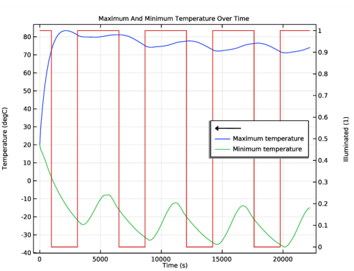
In the Model Builder window, right-click Maximum And Minimum Temperature Over Time and choose Global.
2
In the Settings window for Global, locate the y-Axis Data section.
3
4
Locate the y-Axis section. Select the Plot on secondary y-axis check box.
5
Click to expand the Legends section. Clear the Show legends check box.
Maximum And Minimum Temperature Over Time
1
In the Model Builder window, click Maximum And Minimum Temperature Over Time.
2
In the Maximum And Minimum Temperature Over Time toolbar, click  Plot.