|
|
|
|
•
|
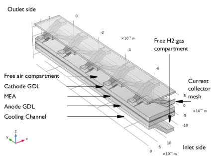
The charge and species balances, reaction and gas phase thermodynamics and the electrochemical reactions are all defined by the use of a Hydrogen Fuel Cell (fc) interface. This interface also includes water permeation and electroosmotic drag through the membrane.
|
|
•
|
The convective flow and pressure of the gas phases in the free gas compartments and the gas diffusion layers (GDLs) are defined by two Free and Porous Media (fp) interfaces, one for each gas mixture. These physics interfaces solve for the Navier-Stokes equations in the free gas domains, and the Brinkman equations in the GDLs.
|
|
•
|
The convective flow and pressure of the liquid cooling fluid is defined using a Laminar Flow (spf) interface. This interface solves for the Navier–Stokes equations.
|
|
•
|
The heat transfer and temperature of the cell is defined and solved for by the use of a Heat Transfer (ht) interface
|
|
•
|
The Reacting Flow nodes, one for each gas phase, applies the convective velocities and pressures of the fp interfaces into the species transport equations and electrochemical reaction kinetics expressions of the fc interface. These coupling nodes also set the density and dynamic viscosity in the fp interfaces to the variables calculated by the fc interface.
|
|
•
|
The Electrochemical Heating node applies the heat sources stemming from the electrochemical reactions and ohmic (joule) heating calculated by the fc interface into the ht interface. The node also sets the temperature in all fc domains to that of the ht interface
|
|
•
|
The Nonisothermal Flow nodes, one for each fluid flow interface, couples the velocity field in the fp and spf interfaces to the fluid domains of the ht interfaces. The node also sets the temperature in all fp and spf domains to that of the ht interface
|
|
•
|
Step 1: Current Distribution Initialization. This study step solves for the potential variables of the fc interface only, for a cell potential of 1 V.
|
|
•
|
|
•
|
Step 5: Stationary - All Physics Except Laminar Flow. This study step starts solving for the full problem at a cell potential of 1 V, ramping it down to 0.5 V by the use of an Auxiliary Sweep. Since the properties of the cooling fluid are not assumed to be affected by changes in temperature, the spf interface is excluded from solving in this study step.
|


|
1
|
|
2
|
|
3
|
Click Add.
|
|
4
|
In the Select Physics tree, select Fluid Flow>Porous Media and Subsurface Flow>Free and Porous Media Flow (fp).
|
|
5
|
Click Add.
|
|
6
|
|
7
|
In the Velocity field components table, enter the following settings:
|
|
8
|
|
9
|
Click Add.
|
|
10
|
|
11
|
In the Velocity field components table, enter the following settings:
|
|
12
|
|
13
|
|
14
|
Click Add.
|
|
15
|
|
16
|
Click Add.
|
|
17
|
|
18
|
In the Velocity field components table, enter the following settings:
|
|
19
|
|
20
|
Click
|
|
21
|
Click
|
|
1
|
|
2
|
|
3
|
|
4
|
|
5
|
Browse to the model’s Application Libraries folder and double-click the file nonisothermal_pem_fuel_cell_geom_sequence.mph.
|
|
6
|
|
1
|
|
2
|
|
1
|
|
2
|
|
3
|
|
4
|
Browse to the model’s Application Libraries folder and double-click the file nonisothermal_pem_fuel_cell_physics_parameters.txt.
|
|
1
|
|
2
|
|
3
|
|
4
|
|
1
|
|
2
|
|
3
|
|
4
|
|
5
|
|
6
|
|
7
|
In the tree, select Fuel Cell and Electrolyzer>Polymer Electrolytes>Nafion, EW 1100, Vapor Equilibrated, Protonated.
|
|
8
|
|
9
|
|
1
|
|
2
|
|
1
|
|
2
|
|
3
|
|
1
|
|
2
|
|
3
|
|
1
|
|
2
|
|
3
|
|
1
|
|
2
|
|
3
|
|
1
|
|
2
|
In the Settings window for Water Absorption-Desorption, H2 Side, locate the Absorption-Desorption Condition section.
|
|
3
|
|
1
|
|
2
|
In the Settings window for Water Absorption-Desorption, O2 Side, locate the Absorption-Desorption Condition section.
|
|
3
|
|
1
|
|
2
|
|
3
|
|
1
|
|
2
|
|
3
|
|
4
|
|
5
|
|
6
|
|
1
|
|
2
|
|
3
|
|
1
|
|
2
|
|
3
|
|
4
|
|
5
|
|
6
|
|
1
|
|
2
|
|
3
|
|
4
|
|
1
|
|
2
|
|
3
|
|
1
|
|
2
|
|
3
|
|
4
|
|
1
|
In the Model Builder window, expand the Component 1 (comp1)>Hydrogen Fuel Cell (fc)>H2 Gas Phase 1 node, then click Initial Values 1.
|
|
2
|
|
3
|
|
4
|
|
5
|
|
1
|
|
2
|
|
3
|
|
1
|
|
2
|
|
3
|
|
1
|
In the Model Builder window, expand the Component 1 (comp1)>Hydrogen Fuel Cell (fc)>O2 Gas Phase 1 node, then click Initial Values 1.
|
|
2
|
|
3
|
|
4
|
|
5
|
|
1
|
|
2
|
|
3
|
|
1
|
|
2
|
|
3
|
|
1
|
|
2
|
|
3
|
|
4
|
|
1
|
|
2
|
In the Settings window for Thin H2 Gas Diffusion Electrode Reaction, locate the Electrode Kinetics section.
|
|
3
|
|
4
|
|
1
|
|
2
|
|
3
|
|
4
|
|
1
|
|
2
|
In the Settings window for Thin O2 Gas Diffusion Electrode Reaction, locate the Electrode Kinetics section.
|
|
3
|
|
4
|
|
5
|
|
1
|
|
2
|
In the Settings window for Free and Porous Media Flow, type Free and Porous Media Flow - Anode in the Label text field.
|
|
3
|
|
4
|
Locate the Physical Model section. From the Compressibility list, choose Compressible flow (Ma<0.3).
|
|
1
|
|
2
|
|
3
|
|
1
|
|
2
|
|
3
|
|
4
|
|
1
|
|
2
|
|
3
|
|
4
|
|
5
|
|
1
|
|
2
|
|
3
|
|
1
|
|
2
|
|
3
|
|
4
|
|
5
|
|
1
|
|
2
|
|
3
|
|
1
|
|
2
|
In the Settings window for Free and Porous Media Flow, type Free and Porous Media Flow - Cathode in the Label text field.
|
|
3
|
|
4
|
Locate the Physical Model section. From the Compressibility list, choose Compressible flow (Ma<0.3).
|
|
1
|
|
2
|
|
3
|
|
1
|
In the Model Builder window, expand the Component 1 (comp1)>Free and Porous Media Flow - Cathode (fp2) node.
|
|
2
|
|
3
|
|
4
|
|
1
|
|
2
|
|
3
|
|
4
|
|
1
|
|
2
|
|
3
|
|
4
|
|
5
|
|
1
|
|
2
|
|
3
|
|
1
|
|
2
|
|
3
|
|
4
|
|
1
|
|
2
|
|
3
|
|
1
|
In the Model Builder window, under Component 1 (comp1)>Heat Transfer in Solids and Fluids (ht) click Fluid 1.
|
|
2
|
|
3
|
|
4
|
Locate the Heat Conduction, Fluid section. From the k list, choose Thermal conductivity, gas phase (fc).
|
|
5
|
|
6
|
|
7
|
|
8
|
|
1
|
|
2
|
|
3
|
|
4
|
Locate the Heat Conduction, Fluid section. From the k list, choose Thermal conductivity, gas phase (fc).
|
|
5
|
|
6
|
|
7
|
|
8
|
|
1
|
|
2
|
|
3
|
|
1
|
|
2
|
|
3
|
|
4
|
Locate the Heat Conduction, Solid section. From the k list, choose User defined. From the list, choose Diagonal.
|
|
5
|
In the k table, enter the following settings:
|
|
6
|
Locate the Thermodynamics, Solid section. From the ρ list, choose User defined. From the Cp list, choose User defined.
|
|
1
|
|
2
|
|
3
|
|
4
|
|
5
|
Locate the Thermodynamics, Solid section. From the ρ list, choose User defined. From the Cp list, choose User defined.
|
|
1
|
|
2
|
|
3
|
|
4
|
|
1
|
|
2
|
|
3
|
|
1
|
|
2
|
|
3
|
|
1
|
|
2
|
|
3
|
|
1
|
|
2
|
|
3
|
|
1
|
|
2
|
|
3
|
|
4
|
|
5
|
|
1
|
|
2
|
|
3
|
|
1
|
|
2
|
|
3
|
|
1
|
|
2
|
In the Settings window for Nonisothermal Flow, type Nonisothermal Flow - Anode Gas in the Label text field.
|
|
1
|
|
2
|
In the Settings window for Nonisothermal Flow, type Nonisothermal Flow - Cathode Gas in the Label text field.
|
|
3
|
Locate the Coupled Interfaces section. From the Fluid flow list, choose Free and Porous Media Flow - Cathode (fp2).
|
|
1
|
|
2
|
In the Settings window for Nonisothermal Flow, type Nonisothermal Flow - Cooling Fluid in the Label text field.
|
|
3
|
|
1
|
In the Model Builder window, under Component 1 (comp1) click Heat Transfer in Solids and Fluids (ht).
|
|
2
|
|
3
|
|
1
|
|
2
|
|
3
|
|
4
|
|
5
|
|
6
|
Click OK.
|
|
7
|
|
1
|
|
2
|
|
3
|
|
4
|
|
5
|
Click OK.
|
|
1
|
|
2
|
|
3
|
|
4
|
|
5
|
|
6
|
Click OK.
|
|
7
|
|
8
|
|
9
|
In the Add dialog box, in the Selections to subtract list, choose Cathode Gas Inlet, Cathode Gas Outlet, Anode Gas Inlet, Anode Gas Outlet, Cooling Inlet, Cooling Outlet, and Right and Left Symmetry Boundaries.
|
|
10
|
Click OK.
|
|
1
|
|
2
|
|
3
|
|
4
|
|
5
|
Click OK.
|
|
1
|
|
2
|
|
3
|
|
4
|
|
5
|
Click OK.
|
|
1
|
|
2
|
|
3
|
|
4
|
|
5
|
|
6
|
|
7
|
|
1
|
|
2
|
|
3
|
|
4
|
|
5
|
|
1
|
|
2
|
|
3
|
|
4
|
|
1
|
|
2
|
|
3
|
Click the Custom button.
|
|
4
|
|
5
|
|
6
|
|
1
|
|
2
|
|
3
|
|
4
|
|
5
|
Click to expand the Corner Settings section. From the Handling of sharp edges list, choose Trimming.
|
|
1
|
|
2
|
|
3
|
|
4
|
|
5
|
|
6
|
|
7
|
|
1
|
|
2
|
|
3
|
|
4
|
|
1
|
|
2
|
|
1
|
|
2
|
|
3
|
Find the Studies subsection. In the Select Study tree, select Preset Studies for Selected Physics Interfaces>Hydrogen Fuel Cell>Stationary with Initialization.
|
|
4
|
|
5
|
|
1
|
|
2
|
|
1
|
|
2
|
|
3
|
|
1
|
|
2
|
|
3
|
|
1
|
|
2
|
In the Settings window for Stationary, type Stationary - All Physics Except Laminar Flow in the Label text field.
|
|
3
|
|
4
|
|
5
|
Click
|
|
1
|
|
2
|
|
3
|
In the Model Builder window, expand the Study 1>Solver Configurations>Solution 1 (sol1)>Stationary Solver 5 node, then click Segregated 1.
|
|
4
|
|
5
|
|
6
|
In the Model Builder window, expand the Study 1>Solver Configurations>Solution 1 (sol1)>Stationary Solver 5>Segregated 1 node, then click Velocity ua, Pressure pa.
|
|
7
|
|
8
|
|
9
|
In the Model Builder window, under Study 1>Solver Configurations>Solution 1 (sol1)>Stationary Solver 5>Segregated 1 click Temperature.
|
|
10
|
|
11
|
|
12
|
In the Model Builder window, under Study 1>Solver Configurations>Solution 1 (sol1)>Stationary Solver 5>Segregated 1 click Velocity uc, Pressure pc.
|
|
13
|
|
14
|
|
15
|
|
1
|
In the Model Builder window, under Study 1 click Step 5: Stationary - All Physics Except Laminar Flow.
|
|
2
|
|
3
|
Select the Plot check box.
|
|
4
|
|
5
|
|
1
|
|
2
|
|
1
|
|
2
|
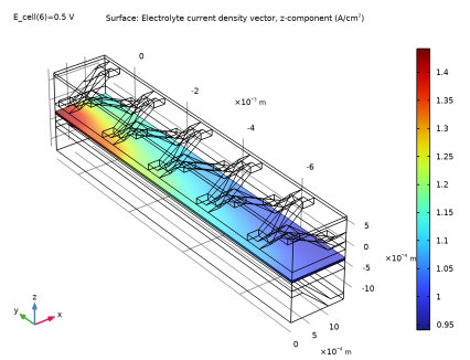
In the Settings window for Surface, click Replace Expression in the upper-right corner of the Expression section. From the menu, choose Component 1 (comp1)>Hydrogen Fuel Cell>Electrolyte current density vector - A/m²>fc.Ilz - Electrolyte current density vector, z-component.
|
|
3
|
|
4
|
|
1
|
|
2
|
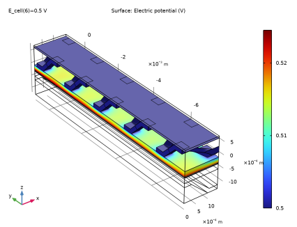
In the Settings window for 3D Plot Group, type Electrode Phase Potential, Anode Side in the Label text field.
|
|
1
|
|
2
|
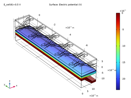
In the Settings window for Surface, click Replace Expression in the upper-right corner of the Expression section. From the menu, choose Component 1 (comp1)>Hydrogen Fuel Cell>fc.phis - Electric potential - V.
|
|
1
|
|
2
|
|
3
|
|
4
|
|
1
|
In the Model Builder window, right-click Electrode Phase Potential, Anode Side and choose Duplicate.
|
|
2
|
In the Settings window for 3D Plot Group, type Electrode Phase Potential, Cathode in the Label text field.
|
|
3
|
|
1
|
In the Model Builder window, expand the Results>Electrode Phase Potential, Cathode>Surface 1 node, then click Selection 1.
|
|
2
|
|
3
|
|
4
|
|
1
|
|
2
|
|
3
|
|
1
|
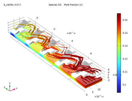
In the Model Builder window, expand the Mole Fraction, O2, Streamline (fc) node, then click Streamline 1.
|
|
2
|
|
3
|
|
4
|
Locate the Streamline Positioning section. From the Positioning list, choose On selected boundaries.
|
|
5
|
|
6
|
|
7
|
Locate the Coloring and Style section. Find the Line style subsection. From the Type list, choose Ribbon.
|
|
1
|
|
2
|
|
3
|
|
1
|
|
2
|
In the Settings window for Surface, click Replace Expression in the upper-right corner of the Expression section. From the menu, choose Component 1 (comp1)>Hydrogen Fuel Cell>Species O2>fc.xO2 - Mole fraction.
|
|
3
|
|
4
|
|
5
|
|
1
|
|
2
|
|
3
|
|
1
|
|
2
|
|
3
|
|
4
|
|
5
|
|
6
|
|
1
|
|
2
|
|
3
|
|
1
|
|
2
|
|
3
|
|
1
|
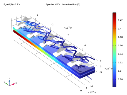
In the Model Builder window, expand the Results>Mole Fraction, H2O, Streamline (fc) node, then click Mole Fraction, H2O, Streamline (fc).
|
|
2
|
|
3
|
|
1
|
|
2
|
|
3
|
|
4
|
Locate the Coloring and Style section. Find the Line style subsection. From the Type list, choose Ribbon.
|
|
1
|
|
2
|
|
3
|
|
1
|
|
2
|
In the Settings window for Surface, click Replace Expression in the upper-right corner of the Expression section. From the menu, choose Component 1 (comp1)>Hydrogen Fuel Cell>Species H2O>fc.xH2O - Mole fraction.
|
|
3
|
|
4
|
|
5
|
|
1
|
|
2
|
|
3
|
|
1
|
|
2
|
|
1
|
|
2
|
|
3
|
|
4
|
|
1
|
|
2
|
|
1
|
|
2
|
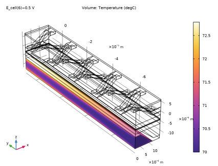
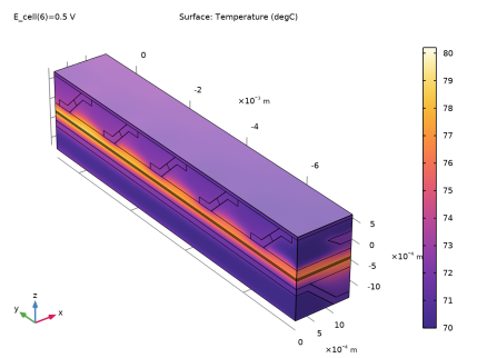
In the Settings window for Volume, click Replace Expression in the upper-right corner of the Expression section. From the menu, choose Component 1 (comp1)>Heat Transfer in Solids and Fluids>Temperature>T - Temperature - K.
|
|
3
|
|
4
|
|
5
|
|
6
|
Click OK.
|
|
1
|
|
2
|
|
3
|
|
4
|
|
1
|
|
2
|
|
1
|
|
2
|
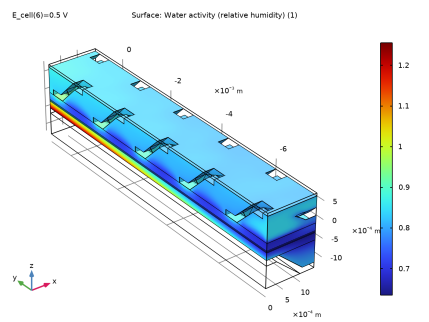
In the Settings window for Surface, click Replace Expression in the upper-right corner of the Expression section. From the menu, choose Component 1 (comp1)>Hydrogen Fuel Cell>fc.aw - Water activity (relative humidity).
|
|
3
|