|
|
|
|
•
|
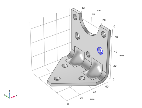
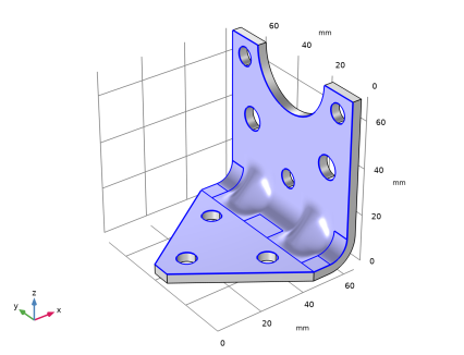
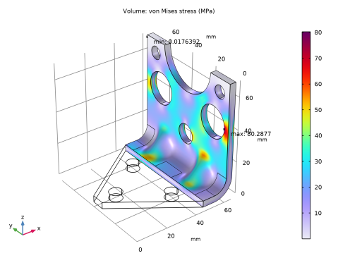
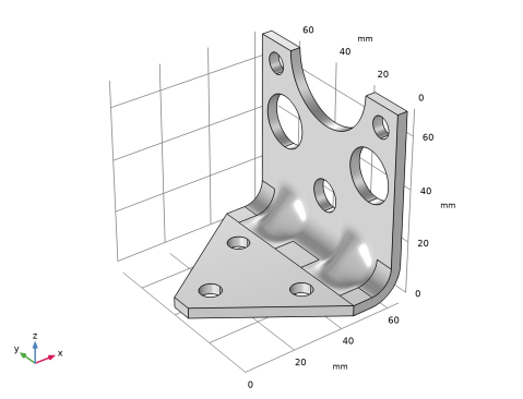
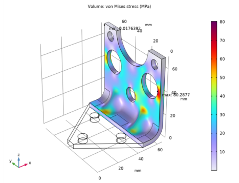
When exposed to a peak acceleration of 4g in all three global directions simultaneously, the effective stress is not allowed to exceed 80 MPa anywhere. This criterion is nondifferentiable because the location of the peak stress can jump from one place to another. A gradient-free optimization algorithm must thus be used.
|
|
1
|
|
2
|
|
3
|
Click Add.
|
|
4
|
Click
|
|
5
|
|
6
|
Click
|
|
1
|
|
2
|
|
3
|
|
4
|
Browse to the model’s Application Libraries folder and double-click the file bracket_import_optimization_dimensions_parameters.txt.
|
|
5
|
|
6
|
|
1
|
|
2
|
|
3
|
|
1
|
|
2
|
|
3
|
Click
|
|
4
|
Browse to the model’s Application Libraries folder and double-click the file bracket_import_optimization_geom.step.
|
|
5
|
|
6
|
|
1
|
|
2
|
|
3
|
|
1
|
|
2
|
|
3
|
|
4
|
|
5
|
|
1
|
|
2
|
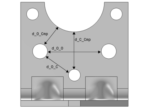
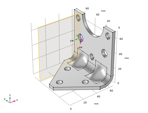
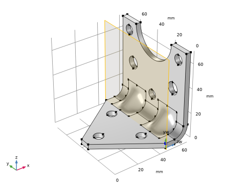
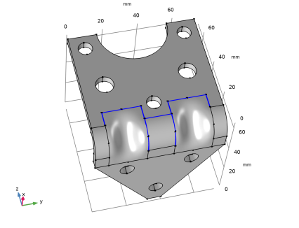
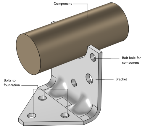
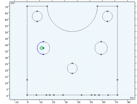
Select the two outer boundaries of the bracket, following the figure below, and apply Distance by clicking on the Graphics window.
 |
|
3
|
In the Settings window for Distance, locate the Dimension Value section. Click to clear the associated Constrain Distance toggle button (lock symbol).
|
|
4
|
Select the Create parameter check box.
|
|
5
|
|
6
|
|
1
|
|
2
|
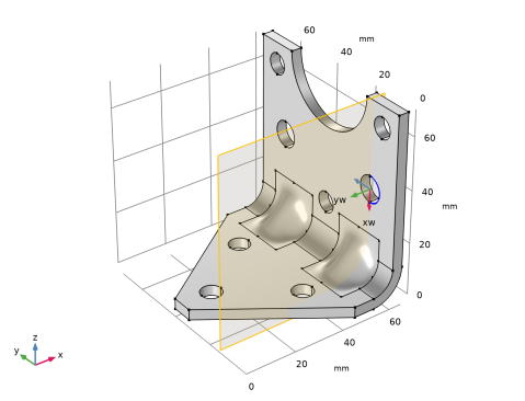
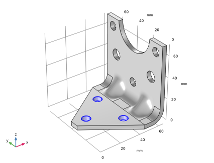
Select the edge of the mounting component hole, following the figure below, and apply Radius by clicking on the Graphics window.
 |
|
3
|
In the Settings window for Radius, locate the Dimension Value section. Click to clear the associated Constrain Radius toggle button (lock symbol).
|
|
4
|
Select the Create parameter check box.
|
|
5
|
|
6
|
|
1
|
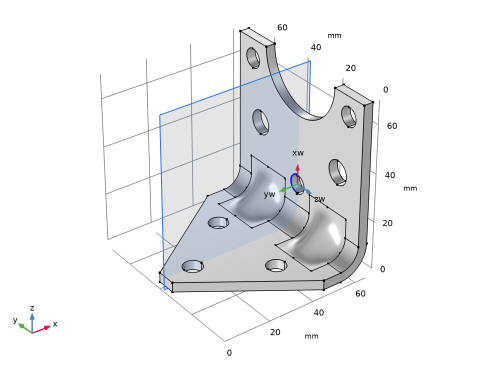
In the Model Builder window, under Component 1>Geometry 1 right-click Original Geometry and choose Work Plane.
|
|
2
|
In the Settings window for Work Plane, type Coordinate System - Central Hole in the Label text field.
|
|
3
|
|
4
|
|
5
|
|
1
|
|
2
|
In the Settings window for Work Plane, type Coordinate System - Outer Hole 1 in the Label text field.
|
|
3
|
|
4
|
|
5
|
|
6
|
|
1
|
|
2
|
In the Settings window for Work Plane, type Coordinate System - Outer Hole 2 in the Label text field.
|
|
3
|
|
4
|
|
5
|
|
1
|
|
2
|
In the Settings window for Transform Faces, type Z Displacement and Scaling - Central Hole in the Label text field.
|
|
3
|
|
4
|
Locate the Coordinate System section. From the Work plane list, choose Coordinate System - Central Hole.
|
|
5
|
|
6
|
|
7
|
|
1
|
|
2
|
|
3
|
|
4
|
|
5
|
|
6
|
|
1
|
|
2
|
In the Settings window for Transform Faces, type Displacement - Outer Hole 1 in the Label text field.
|
|
3
|
|
4
|
Locate the Coordinate System section. From the Work plane list, choose Coordinate System - Outer Hole 1.
|
|
5
|
|
6
|
|
7
|
|
1
|
|
2
|
In the Settings window for Transform Faces, type Displacement - Outer Hole 2 in the Label text field.
|
|
3
|
|
4
|
Locate the Coordinate System section. From the Work plane list, choose Coordinate System - Outer Hole 2.
|
|
5
|
|
6
|
|
7
|
|
1
|
|
2
|
|
3
|
|
4
|
|
5
|
|
6
|
|
7
|
|
1
|
|
2
|
Select the object tf3 only.
|
|
3
|
|
4
|
|
5
|
|
1
|
|
2
|
|
3
|
|
1
|
|
2
|
|
3
|
Find the In-plane visualization of 3D geometry subsection. Clear the Coincident entities (blue) check box.
|
|
4
|
|
5
|
|
1
|
|
2
|
|
3
|
|
4
|
|
1
|
|
2
|
|
3
|
|
1
|
|
2
|
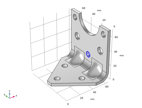
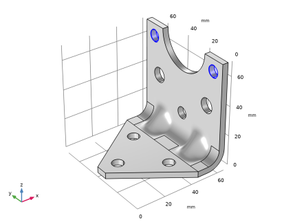
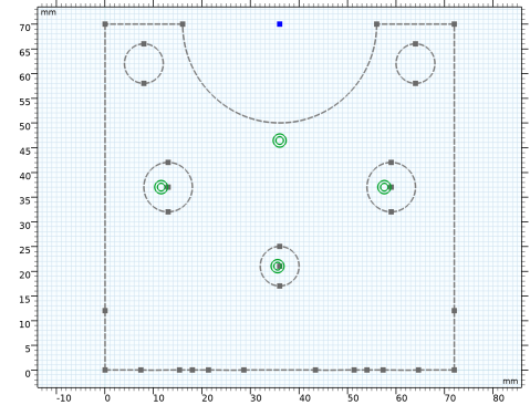
Select one edge of the left outer hole and Point 1 and apply the Concentric constraint by clicking on the Graphics window.
 |
|
1
|
|
2
|
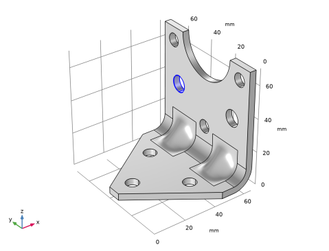
Select the point in the left outer hole and the mounting component and apply Distance by clicking on the Graphics window.
|
|
3
|
In the Settings window for Distance, locate the Dimension Value section. Click to clear the associated Constrain Distance toggle button (lock symbol).
|
|
4
|
Select the Create parameter check box.
|
|
5
|
|
1
|
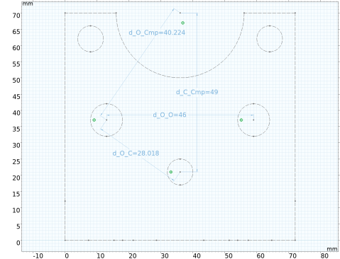
Add three more Distance constraints by following the steps in the section above to create the following dimension parameters.
|
|
1
|
|
2
|
|
3
|
|
4
|
|
5
|
|
1
|
|
2
|
|
3
|
|
4
|
|
5
|
|
1
|
|
2
|
|
3
|
|
4
|
|
5
|
|
1
|
|
2
|
|
3
|
|
4
|
|
5
|
|
1
|
|
2
|
|
3
|
|
4
|
|
5
|
|
6
|
|
7
|
|
8
|
|
9
|
|
10
|
|
11
|
|
12
|
Click OK.
|
|
13
|
|
1
|
|
2
|
|
3
|
|
4
|
|
5
|
|
6
|
|
7
|
|
8
|
|
9
|
|
10
|
Locate the Resulting Selection section. Find the Cumulative selection subsection. From the Contribute to list, choose Ignore Edges Selection.
|
|
11
|
|
1
|
|
2
|
|
3
|
|
4
|
|
5
|
|
6
|
|
7
|
|
8
|
|
9
|
|
10
|
Locate the Resulting Selection section. Find the Cumulative selection subsection. From the Contribute to list, choose Ignore Edges Selection.
|
|
11
|
|
1
|
|
2
|
|
3
|
|
4
|
|
5
|
|
1
|
|
2
|
|
3
|
|
4
|
|
5
|
|
1
|
In the Model Builder window, under Component 1 right-click Solid Mechanics and choose Fixed Constraint.
|
|
2
|
|
1
|
|
2
|
In the Settings window for Rigid Connector, type Rigid Connector (Mounted component) in the Label text field.
|
|
4
|
|
5
|
|
1
|
|
2
|
In the Settings window for Mass and Moment of Inertia, locate the Mass and Moment of Inertia section.
|
|
3
|
|
4
|
From the list, choose Diagonal.
|
|
5
|
In the I table, enter the following settings:
|
|
1
|
|
1
|
|
2
|
|
3
|
|
5
|
|
1
|
|
3
|
|
4
|
|
5
|
|
1
|
|
2
|
|
3
|
|
4
|
|
1
|
|
2
|
|
3
|
|
1
|
|
2
|
|
3
|
|
4
|
|
1
|
|
2
|
In the Settings window for Applied Force, type Force 4g on mounted component in the Label text field.
|
|
3
|
|
1
|
|
2
|
|
3
|
|
4
|
|
5
|
|
1
|
|
2
|
|
3
|
|
1
|
|
2
|
|
1
|
|
2
|
|
3
|
|
4
|
Click Replace Expression in the upper-right corner of the Expression section. From the menu, choose Component 1>Solid Mechanics>Material properties>solid.rho - Density - kg/m³.
|
|
1
|
|
2
|
|
3
|
|
4
|
|
5
|
Click Replace Expression in the upper-right corner of the Expression section. From the menu, choose Component 1>Solid Mechanics>Stress>solid.mises - von Mises stress - N/m².
|
|
1
|
|
2
|
|
1
|
|
2
|
|
3
|
|
1
|
|
2
|
|
1
|
|
2
|
|
3
|
|
1
|
|
2
|
|
1
|
|
2
|
|
3
|
|
4
|
|
5
|
|
1
|
|
2
|
|
3
|
|
1
|
|
2
|
|
3
|
|
1
|
|
2
|
|
3
|
|
4
|
|
5
|
|
6
|
Click Replace Expression in the upper-right corner of the Objective Function section. From the menu, choose Component 1>Definitions>comp1.mass - Domain Probe 1 - kg.
|
|
7
|
|
8
|
|
9
|
|
10
|
Browse to the model’s Application Libraries folder and double-click the file bracket_import_optimization_ctrlvars.txt.
|
|
11
|
Locate the Constraints section. In the table, enter the following settings:
|
|
12
|
|
13
|
|
1
|
|
2
|
Click
|
|
1
|
|
2
|
|
1
|
In the Objective Table 3 table, right-click the last row and select Copy Selected Rows to New Parameter Cases.
|
|
1
|
|
2
|
|
3
|
|
4
|