PDF

Galvanic Corrosion with Electrode Deformation
Introduction
This example models the galvanic corrosion and deformation of a magnesium alloy (AE44) in contact with mild steel in brine solution. While similar to the Galvanic Corrosion of a Magnesium Alloy in Contact with Steel example, the present model also investigates the deformation of the corroding electrode over time.
The example is based on a paper by Deshpande (Ref. 1).
Model Definition
The model geometry is shown in Figure 1. Use one single electrolyte domain. The left part of the bottom boundary is the surface of the mild steel material, the right part is the corroding magnesium alloy. Because the alloy corrodes in the model, the right boundary is displaced downward in the geometry. Introduce a small height step of 0.1 mm in the negative y direction at the origin in the geometry to ensure that the topology of the geometry is preserved during the simulation. Let the vertical boundary of the step belong to the steel surface.
Figure 1: Model geometry.
The electrolyte is well mixed so that a secondary current distribution can be assumed, solving for the electrolyte potential,  (V), in the domain. Set the electrolyte conductivity to 5 S/m.
The magnesium alloy is an anode of the galvanic couple, oxidizing magnesium according to
The alloy consists mainly of magnesium, the oxidation reactions of the other alloying elements are neglected in this model.
The mild steel acts as a cathode for this galvanic couple.
The electrode kinetics at both the mild steel and magnesium alloy surfaces is described using the experimental polarization data available in corrosion material library.
The dissolution of magnesium metal causes the electrode boundary to move, with a velocity in the normal direction, v (SI unit: m/s), according to
where ian (SI unit: A/m2) is the anodic electrode reaction current density, M is the mean molar mass (25 g/mol) and ρ the density (1820 kg/m3) of the magnesium alloy.
Solve the model in a time-dependent study, simulating the corrosion for three days of immersion in salt water.
Results and Discussion
Figure 2 shows the electrode current densities at the beginning and the end of the simulation. As expected, the highest electrode current densities are found at the contact point between the two metals.
Figure 2: Electrode current densities at t = 0 and t = 72 h.
Figure 3 shows the current density and potential distribution in the electrolyte, and the model geometry, at the beginning of the simulation.
Figure 3: Model geometry, electrolyte potential, and current densities at t = 0.
Figure 4 shows the current density and potential distribution in the electrolyte and the changed geometry at the end of the simulation. Because the electrode current densities are highest at the contact point of the metals, the metal dissolution is also maximum at this point. When compared to Figure 3, the electrolyte potential is quite similar, which matches the results of Figure 2 with quite similar electrode current densities at the beginning and the end of the simulation.
Figure 4: Model geometry, electrolyte potential, and current densities after 72 h.
Notes About the COMSOL Implementation
Use the Corrosion, Secondary entry from the Model Wizard for this model. It is a predefined multiphysics interface that contains a Secondary Current Distribution interface and a Deformed Geometry node. The Deformed Geometry node handles the deformed geometry (moving mesh/ALE) part of the problem.
For the mild steel surface, which is not deforming, use an Electrode Surface node to model the reduction reaction. For the magnesium alloy surface, use an Electrode Surface node with an added Dissolving-Depositing species, which sets up both the deformation of the geometry and the magnesium electrode reaction. Set the two electrode surfaces to the same electric potential in the metal phase.
Change the boundary condition setting of the default Non-Deforming Boundary node to Zero normal displacement. This imposes pointwise (instead of weak) constraints on the geometry displacement, and thereby fix the corners of the geometry.
Solve the model using a time-dependent study with automatic remeshing enabled.
Reference
1. K.B. Deshpande, “Validated numerical modelling of galvanic corrosion for couples: Magnesium alloy (AE44)-mild steel and AE44-aluminium alloy (AA6063) in brine solution”, Corrosion Science, vol. 52, pp. 3514–3522, 2010.
Application Library path: Corrosion_Module/Galvanic_Corrosion/galvanic_corrosion_with_deformation
Modeling Instructions
From the File menu, choose New.
New
In the New window, click  Model Wizard.
Model Wizard
1
In the Model Wizard window, click  2D.
2
In the Select Physics tree, select Electrochemistry>Corrosion, Deformed Geometry>Corrosion, Secondary.
3
Click Add.
4
Click  Study.
5
In the Select Study tree, select Preset Studies for Selected Physics Interfaces>Time Dependent with Initialization.
6
Geometry 1
Create the model geometry as a union of two rectangles.
Rectangle 1 (r1)
1
In the Geometry toolbar, click  Rectangle.
2
In the Settings window for Rectangle, locate the Size and Shape section.
3
In the Width text field, type 0.01.
4
In the Height text field, type 0.01.
5
Locate the Position section. In the x text field, type -0.01.
Rectangle 2 (r2)
1
In the Geometry toolbar, click  Rectangle.
2
In the Settings window for Rectangle, locate the Size and Shape section.
3
In the Width text field, type 0.01.
4
In the Height text field, type 0.01+1e-4.
5
Locate the Position section. In the y text field, type -1e-4.
Union 1 (uni1)
1
In the Geometry toolbar, click  Booleans and Partitions and choose Union.
2
Click in the Graphics window and then press Ctrl+A to select both objects.
3
In the Settings window for Union, locate the Union section.
4
Clear the Keep interior boundaries check box.
5
In the Geometry toolbar, click  Build All.
6
Click the  Zoom Extents button in the Graphics toolbar.
Global Definitions
Load the model parameters from a text file.
Parameters 1
1
In the Model Builder window, under Global Definitions click Parameters 1.
2
In the Settings window for Parameters, locate the Parameters section.
3
Click  Load from File.
4
Materials
Use the Corrosion Material Library to set up the material properties for the electrode kinetics at the magnesium and mild steel electrode surfaces.
Add Material
1
In the Home toolbar, click  Add Material to open the Add Material window.
2
Go to the Add Material window.
3
In the tree, select Corrosion>Iron Alloys (Steels)>Mild steel in 1.6 wt% NaCl.
4
Click Add to Component in the window toolbar.
Materials
Mild steel in 1.6 wt% NaCl (mat1)
1
In the Settings window for Material, locate the Geometric Entity Selection section.
2
From the Geometric entity level list, choose Boundary.
3
4
In the Model Builder window, expand the Mild steel in 1.6 wt% NaCl (mat1) node.
Interpolation 1 (iloc_exp)
1
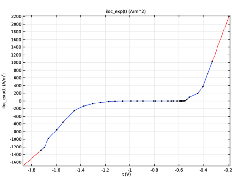
In the Model Builder window, expand the Component 1 (comp1)>Materials>Mild steel in 1.6 wt% NaCl (mat1)>Local current density (lcd) node, then click Interpolation 1 (iloc_exp).
2
In the Settings window for Interpolation, click  Plot.
The function plot should look like this:
Add Material
1
Go to the Add Material window.
2
In the tree, select Corrosion>Magnesium Alloys>AE44 in 1.6 wt% NaCl.
3
Click Add to Component in the window toolbar.
Materials
AE44 in 1.6 wt% NaCl (mat2)
1
In the Settings window for Material, locate the Geometric Entity Selection section.
2
From the Geometric entity level list, choose Boundary.
3
4
In the Model Builder window, expand the AE44 in 1.6 wt% NaCl (mat2) node.
Interpolation 1 (iloc_exp)
1
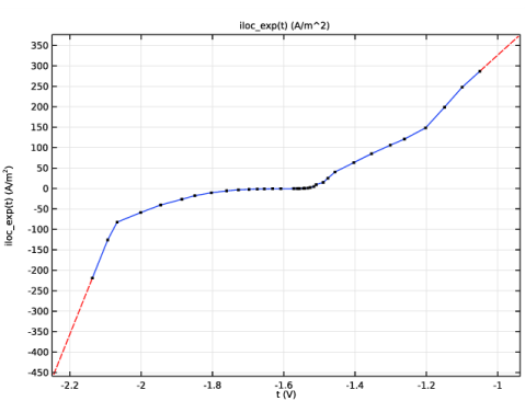
In the Model Builder window, expand the Component 1 (comp1)>Materials>AE44 in 1.6 wt% NaCl (mat2)>Local current density (lcd) node, then click Interpolation 1 (iloc_exp).
2
In the Settings window for Interpolation, click  Plot.
The function plot should look like this:
3
In the Home toolbar, click  Add Material to close the Add Material window.
Secondary Current Distribution (cd)
Now set up the physics for the current distribution. Start with selecting the reference electrode potential.
1
In the Settings window for Secondary Current Distribution, click to expand the Physics vs. Materials Reference Electrode Potential section.
2
From the list, choose 0.241 V (SCE vs. SHE).
Electrolyte 1
Set user defined electrolyte conductivity at the electrolyte domain.
1
In the Model Builder window, under Component 1 (comp1)>Secondary Current Distribution (cd) click Electrolyte 1.
2
In the Settings window for Electrolyte, locate the Electrolyte section.
3
From the σl list, choose User defined. In the associated text field, type sigma.
Electrode Surface 1
The following steps set up the cathodic reduction reaction.
1
In the Physics toolbar, click  Boundaries and choose Electrode Surface.
2
Electrode Reaction 1
1
In the Model Builder window, click Electrode Reaction 1.
2
In the Settings window for Electrode Reaction, locate the Electrode Kinetics section.
3
From the iloc,expr list, choose From material.
Electrode Surface 2
The following steps set up the anodic corrosion reaction and the resulting boundary movement.
1
In the Physics toolbar, click  Boundaries and choose Electrode Surface.
2
3
In the Settings window for Electrode Surface, click to expand the Dissolving-Depositing Species section.
4
5
Electrode Reaction 1
1
In the Model Builder window, click Electrode Reaction 1.
2
In the Settings window for Electrode Reaction, locate the Stoichiometric Coefficients section.
3
In the n text field, type 2.
4
In the Stoichiometric coefficients for dissolving-depositing species: table, enter the following settings:
5
Locate the Electrode Kinetics section. From the iloc,expr list, choose From material.
Multiphysics
Nondeforming Boundary 1 (ndbdg1)
The following applies a stronger constraint (than the default condition) for the planar nondepositing walls in order to enforce a zero boundary movement in the normal direction.
1
In the Model Builder window, under Component 1 (comp1)>Multiphysics click Nondeforming Boundary 1 (ndbdg1).
2
In the Settings window for Nondeforming Boundary, locate the Nondeforming Boundary section.
3
From the Boundary condition list, choose Zero normal displacement.
Deforming Electrode Surface 1 (desdg1)
1
In the Model Builder window, click Deforming Electrode Surface 1 (desdg1).
2
In the Settings window for Deforming Electrode Surface, locate the Boundary Selection section.
3
4
Click  Remove from Selection.
5
Study 1
The simulation time is 72 h.
Step 2: Time Dependent
1
In the Model Builder window, under Study 1 click Step 2: Time Dependent.
2
In the Settings window for Time Dependent, locate the Study Settings section.
3
In the Output times text field, type range(0, 12*3600, 3*24*3600).
4
Click to expand the Study Extensions section. Select the Automatic remeshing check box.
5
In the Home toolbar, click  Compute.
Results
The following reproduces the figures in the Results and Discussion section.
Electrolyte Potential (cd)
1
Click the  Zoom Extents button in the Graphics toolbar.
2
In the Settings window for 2D Plot Group, locate the Plot Settings section.
3
Clear the Plot dataset edges check box.
Line 1
1
Right-click Electrolyte Potential (cd) and choose Line.
2
In the Settings window for Line, locate the Expression section.
3
In the Expression text field, type 1.
4
Locate the Coloring and Style section. From the Coloring list, choose Uniform.
5
From the Color list, choose Black.
6
In the Electrolyte Potential (cd) toolbar, click  Plot.
Electrolyte Potential (cd)
1
In the Model Builder window, click Electrolyte Potential (cd).
2
In the Settings window for 2D Plot Group, locate the Data section.
3
From the Time (s) list, choose 0.
4
In the Electrolyte Potential (cd) toolbar, click  Plot.
1D Plot Group 5
In the Home toolbar, click  Add Plot Group and choose 1D Plot Group.
Line Graph 1
1
Right-click 1D Plot Group 5 and choose Line Graph.
2
In the Settings window for Line Graph, locate the Data section.
3
From the Dataset list, choose Study 1/Remeshed Solution 1 (sol3).
4
From the Time selection list, choose First.
5
6
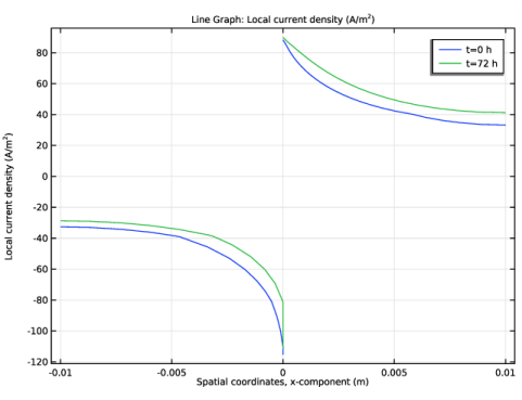
Click Replace Expression in the upper-right corner of the y-Axis Data section. From the menu, choose Component 1 (comp1)>Secondary Current Distribution>Electrode kinetics>cd.iloc_er1 - Local current density - A/m².
7
Locate the x-Axis Data section. From the Parameter list, choose Expression.
8
In the Expression text field, type x.
9
Click to expand the Legends section. Select the Show legends check box.
10
From the Legends list, choose Manual.
11
Line Graph 2
1
Right-click Line Graph 1 and choose Duplicate.
2
In the Settings window for Line Graph, locate the Data section.
3
From the Time selection list, choose Last.
4
Click to expand the Title section. From the Title type list, choose None.
5
Locate the Legends section. In the table, enter the following settings:
6
In the 1D Plot Group 5 toolbar, click  Plot.