PDF

Galvanic Corrosion of a Magnesium Alloy in Contact with Steel
Introduction
Magnesium alloys are attractive alternatives as lightweight materials in various fields of engineering. Magnesium is however relatively non-noble and may suffer considerable galvanic corrosion when being used in conjunction with other metals, for instance when mounting a Mg alloy component using steel fasteners.
This model example simulates a galvanic corrosion couple consisting of a magnesium alloy (AZ91D) and steel (4150), with salt water (5% NaCl) as electrolyte. The example is based on a paper by J.X. Jia and others (Ref. 1).
Model Definition
The model is made in two dimensions using axial symmetry, see Figure 1, with a single electrolyte domain of radius 10 cm and height of 7.5 cm. The electrolyte conductivity is set to 7.95 S/m.
Figure 1: Model geometry. Electrolyte domain with axial symmetry.
Boundary conditions
The cathode is a disc made of steel 4150, placed at the center of the geometry at z=0, extending in the r direction. Three different disc radii are investigated: 5, 10, and 30 mm.
The Mg alloy AZ91D electrode is placed outside the steel disc on the z = 0 line.
The electrode kinetics at both the steel and Mg alloy surfaces is described using the experimental polarization data available in corrosion material library.
The electric potential of both electrode surfaces is set to ground.
The outer (r = 10 cm) and top boundaries (z = 7.5 cm) are insulated.
Results and Discussion
Figure 2 shows a revolved surface plot of the electrolyte potential for a disc radius of 30 mm.
Figure 2: Electrolyte potential for a 30 mm disc radius.
Figure 3 shows the electrode current densities for the three different disc radii. The local current density of the anode reaction in the vicinity of the steel disc increases significantly with an increase in steel disc radius which is attributed to the higher cathode to anode area ratio.
Figure 3: Electrode current densities for the three different disc radii.
Notes About the COMSOL Implementation
The Secondary Current Distribution interface is used to model the problem, using Electrode Surface nodes for the two electrode surfaces.
Due to the faster kinetics and larger area of the anode, the initial value for the electrolyte is set to correspond to a zero anode polarization.
A stationary study step is used to solve the problem, with a parametric sweep to vary the disc radius.
A free triangular mesh is used for meshing, with an additional smaller size setting for increasing the resolution at the contact point between the anode and cathode.
Reference
1. J.X. Jia, A. Atrens, G. Song, and T.H. Muster, “Simulation of galvanic corrosion of magnesium coupled to a steel fastener in NaCl solution,” Materials and Corrosion, vol. 56, no. 7, pp. 468–474, 2005.
Application Library path: Corrosion_Module/Galvanic_Corrosion/galvanic_corrosion_mg_alloy
Modeling Instructions
From the File menu, choose New.
New
In the New window, click  Model Wizard.
Model Wizard
1
In the Model Wizard window, click  2D Axisymmetric.
2
In the Select Physics tree, select Electrochemistry>Primary and Secondary Current Distribution>Secondary Current Distribution (cd).
3
Click Add.
4
Click  Study.
5
In the Select Study tree, select General Studies>Stationary.
6
Global Definitions
Load the model parameters from a file.
Parameters 1
1
In the Model Builder window, under Global Definitions click Parameters 1.
2
In the Settings window for Parameters, locate the Parameters section.
3
Click  Load from File.
4
Geometry 1
Draw the geometry as a rectangle. Use a point to divide the bottom boundary into two sections. (The two sections will be the anode and cathode, respectively, when setting up the physics).
Rectangle 1 (r1)
1
In the Geometry toolbar, click  Rectangle.
2
In the Settings window for Rectangle, locate the Size and Shape section.
3
In the Width text field, type R_outer.
4
In the Height text field, type H.
5
Click  Build Selected.
Point 1 (pt1)
1
In the Geometry toolbar, click  Point.
2
In the Settings window for Point, locate the Point section.
3
In the r text field, type R_inner.
4
Click  Build Selected.
5
Click the  Zoom Extents button in the Graphics toolbar.
Materials
Use the Corrosion Material Library to set up the material properties for the electrode kinetics at the magnesium and steel electrode surfaces.
Add Material
1
In the Home toolbar, click  Add Material to open the Add Material window.
2
Go to the Add Material window.
3
In the tree, select Corrosion>Iron Alloys (Steels)>AISI 4150 steel in 5% NaCl.
4
Click Add to Component in the window toolbar.
Materials
AISI 4150 steel in 5% NaCl (mat1)
1
In the Settings window for Material, locate the Geometric Entity Selection section.
2
From the Geometric entity level list, choose Boundary.
3
4
In the Model Builder window, expand the AISI 4150 steel in 5% NaCl (mat1) node.
Interpolation 1 (iloc_exp)
1
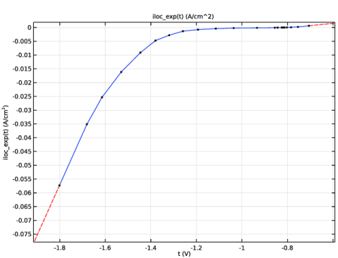
In the Model Builder window, expand the Component 1 (comp1)>Materials>AISI 4150 steel in 5% NaCl (mat1)>Local current density (lcd) node, then click Interpolation 1 (iloc_exp).
2
In the Settings window for Interpolation, click  Plot.
The function plot should look like this:
Add Material
1
Go to the Add Material window.
2
In the tree, select Corrosion>Magnesium Alloys>AZ91D in 5% NaCl.
3
Click Add to Component in the window toolbar.
Materials
AZ91D in 5% NaCl (mat2)
1
In the Settings window for Material, locate the Geometric Entity Selection section.
2
From the Geometric entity level list, choose Boundary.
3
4
In the Model Builder window, expand the AZ91D in 5% NaCl (mat2) node.
Interpolation 1 (iloc_exp)
1
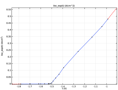
In the Model Builder window, expand the Component 1 (comp1)>Materials>AZ91D in 5% NaCl (mat2)>Local current density (lcd) node, then click Interpolation 1 (iloc_exp).
2
In the Settings window for Interpolation, click  Plot.
The function plot should look like this:
3
In the Home toolbar, click  Add Material to close the Add Material window.
Secondary Current Distribution (cd)
Now set up the electrochemistry. Start with selecting the reference electrode.
1
In the Settings window for Secondary Current Distribution, click to expand the Physics vs. Materials Reference Electrode Potential section.
2
From the list, choose 0.197 V (Sat. Ag/AgCl vs. SHE).
Electrolyte 1
Next set up the user defined electrolyte conductivity.
1
In the Model Builder window, under Component 1 (comp1)>Secondary Current Distribution (cd) click Electrolyte 1.
2
In the Settings window for Electrolyte, locate the Electrolyte section.
3
From the σl list, choose User defined. In the associated text field, type sigma.
Electrode Surface 1
The anode and cathode are modeled as Electrode Surface nodes, having the same electric potential in the electron conducting phase. Define the cathode first.
1
In the Physics toolbar, click  Boundaries and choose Electrode Surface.
The cathode is located at the center of the bottom boundary.
2
Electrode Reaction 1
1
In the Model Builder window, click Electrode Reaction 1.
2
In the Settings window for Electrode Reaction, locate the Electrode Kinetics section.
3
From the iloc,expr list, choose From material.
Electrode Surface 2
Now define the anode surface, located on the outer part of the bottom boundary.
1
In the Physics toolbar, click  Boundaries and choose Electrode Surface.
2
Electrode Reaction 1
1
In the Model Builder window, click Electrode Reaction 1.
2
In the Settings window for Electrode Reaction, locate the Electrode Kinetics section.
3
From the iloc,expr list, choose From material.
Study 1
The model is now ready to solve. Add a parametric sweep to study the impact of different cathode radii.
Parametric Sweep
1
In the Study toolbar, click  Parametric Sweep.
2
In the Settings window for Parametric Sweep, locate the Study Settings section.
3
4
5
In the Study toolbar, click  Compute.
Results
Electrolyte Potential, 3D (cd)
A revolved plot of the electrolyte potential is added by default.
Local current density
The following steps create a plot of the electrode reaction currents. (Compare with Figure 3 in the Results and Discussion section above).
1
In the Home toolbar, click  Add Plot Group and choose 1D Plot Group.
2
In the Settings window for 1D Plot Group, type Local current density in the Label text field.
3
Locate the Data section. From the Dataset list, choose Study 1/Parametric Solutions 1 (sol2).
4
Click to expand the Title section. From the Title type list, choose None.
Line Graph 1
1
Right-click Local current density and choose Line Graph.
2
3
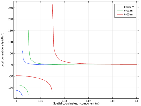
In the Settings window for Line Graph, click Replace Expression in the upper-right corner of the y-Axis Data section. From the menu, choose Component 1 (comp1)>Secondary Current Distribution>Electrode kinetics>cd.iloc_er1 - Local current density - A/m².
4
Locate the x-Axis Data section. From the Parameter list, choose Expression.
5
In the Expression text field, type r.
6
Click to expand the Legends section. Select the Show legends check box.
7
In the Local current density toolbar, click  Plot.