PDF

Atmospheric Corrosion of a Busbar
Introduction
In this model example, the Atmospheric Corrosion model is extended to a busbar which is a metallic strip typically used for high current power distribution. The busbar geometry considered here consists of a copper (Cu) flange, an aluminum (Al) flange and a zinc nut and bolt and is exposed to humidified air.
This tutorial model example solves for both the electric potential in electrode domain and the electrolyte potential in the thin electrolyte layer. A high current is applied at the Cu terminal and the Al terminal is grounded while solving for the electric potential. The electrolyte potential variation is solved only over the exterior surfaces of the busbar geometry. The electrolyte film thickness and conductivity depend on the relative humidity of the surrounding air. The limiting oxygen reduction current density depends on the oxygen diffusivity and solubility.
The example uses parameter data from Ref. 1, Ref. 2, and Ref. 3.
Model Definition
The model setup is shown in Figure 1.
Figure 1: Model setup. The busbar geometry consists of a copper flange, an aluminum flange and a zinc nut and bolt.
The busbar model geometry consists of a copper flange, an aluminum flange, and a zinc nut and bolt. Use the Secondary Current Distribution interface to solve for the electric potential, φs (SI unit: V), over the metal electrode domains of aluminum, copper, and zinc according to:
where is (SI unit: A/m2) is the electrode current density vector and σs (SI unit: S/m) is the electrical conductivity which is assumed to be a constant for all the three domains.
The aluminum terminal is grounded where as total current of 100 A is applied at the copper terminal.
Use the Current Distribution, Shell interface to solve for the electrolyte potential, φl (SI unit: V), over the thin electrolyte domain (over the exterior surfaces of the busbar geometry) according to:
where il (SI unit: A/m2) is the electrolyte current density vector, s (SI unit: m) the electrolyte film thickness and σl (SI unit: S/m) is the electrolyte conductivity which depends on relative humidity.
The thickness of the electrolyte film depends on both the salt load density and the relative humidity. The oxygen solubility and the electrolyte conductivity also depend on the relative humidity. The same expressions as used in the Atmospheric Corrosion model are used here for the electrolyte film thickness, oxygen solubility and electrolyte conductivity to account for the relative humidity dependence. The oxygen diffusivity is assumed to constant in this model.
Electrochemical Reactions
The aluminum, copper, and zinc surfaces account for both the metal dissolution reaction and the oxygen reduction reaction. The metal dissolution electrode reaction kinetics is described by a Anodic Tafel expression whereas the oxygen reduction electrode kinetics is described by a Cathodic Tafel expression.
The oxygen reduction reaction is limited by oxygen transport through the film. The limiting current density, ilim, O2 (SI unit: A/m2), depends on the film thickness, the oxygen solubility and the oxygen diffusivity according to:
where F (96485 C/mol) is Faraday’s constant, D (SI unit: m2/s) is the diffusivity of oxygen in the film, csol (SI unit: mol/m3) is the solubility of oxygen, and dfilm (SI unit: m) is the film thickness.
By assuming a first order dependency of the oxygen reduction kinetics on the local current density of the oxygen concentration, the following expression for the current density, ilim, O2 (SI unit: A/m2), can be derived:
where iexpr is the local current density of the electrode reaction in absence of mass transport limitations.
Results and Discussion
Figure 2 shows the electric potential variation in the metal. It can be seen that the applied current of 100 A is causing a potential drop of about 2.5 mV over the busbar.
Figure 2: The electric potential in the metal.
Figure 3 shows the variation in electrode potential versus adjacent reference, which is the difference between the electric potential in the metal and the electrolyte film potential. The electrode potential versus adjacent reference is positive over the copper flange and negative over the zinc nut and bolt and aluminum flange surfaces.
Figure 3: The electrode potential vs. adjacent reference.
Figure 4 shows the electrolyte potential variation in the electrolyte film.
Figure 4: The electrolyte potential obtained in the electrolyte film covering the busbar.
Figure 5 shows the local current density variation for the anodic metal dissolution reaction. It can be seen that the metal dissolution electrode reaction predominantly occurs near the intersection region between the copper flange and the zinc bolt, at the zinc surface. (Zooming and rotating the plot in the model file also reveals metal dissolution occurring between the copper flange and aluminum flange at the aluminum surface.)
Figure 5: The local current density for metal dissolution electrode reaction over the exterior busbar surfaces.
Finally, Figure 6 shows the local current density variation for the oxygen reduction electrode reaction over the exterior surfaces of the busbar. It can be seen that the oxygen reduction electrode reaction predominantly occurs on the aluminum and zinc surfaces. The magnitude of local oxygen reduction current density is close to the limiting current density, indicating that transport of oxygen is limiting the corrosion process.
Figure 6: The local current density for oxygen reduction electrode reaction over the exterior surfaces of the busbar.
Notes About the COMSOL Implementation
The model is implemented using the Secondary Current Distribution interface to solve for the electric potential and the Current Distribution, Shell interface to solve for the electrolyte potential in the thin electrolyte film. Note that the Current Distribution, Shell interface is only applicable to the exterior boundary selections of the busbar domain.
References
1. Z.Y. Chen, F. Cui, and R.G. Kelly, “Calculations of the Cathodic Current Delivery Capacity and Stability of Crevice Corrosion under Atmospheric Environments”, J. Electrochemical Society, vol. 155, no. 7, pp. C360–368, 2008.
2. D. Mizuno and R.G. Kelly “Galvanically Induced Intergranular Corrosion of AA5083-H131 Under Atmospheric Exposure Conditions — Part II — Modeling of the Damage Distribution”, Corrosion, vol. 69, no. 6, pp. 580–592, 2013.
3. D. Mizuno, Y. Shi, and R.G. Kelly, “Modeling of Galvanic Interactions between AA5083 and Steel under Atmospheric Conditions”, Excerpt from the Proceedings of the 2011 COMSOL Conference in Boston.
Application Library path: Corrosion_Module/Atmospheric_Corrosion/atmospheric_corrosion_busbar
Modeling Instructions
Begin by loading the model geometry file which also includes customized selections.
Application Libraries
1
From the File menu, choose Application Libraries.
2
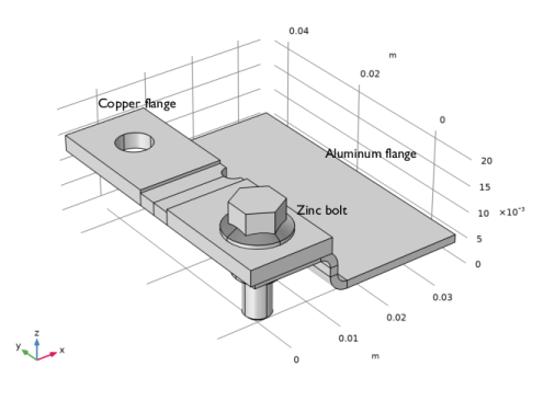
In the Application Libraries window, select Corrosion Module>Atmospheric Corrosion>atmospheric_corrosion_busbar_geom in the tree.
3
Add Physics
1
In the Home toolbar, click  Add Physics to open the Add Physics window.
Add physics interfaces Secondary Current Distribution to solve for the electric potential and Current Distribution, Shell to solve for the electrolyte potential.
2
Go to the Add Physics window.
3
In the tree, select Electrochemistry>Primary and Secondary Current Distribution>Secondary Current Distribution (cd).
4
Click Add to Component 1 in the window toolbar.
5
In the tree, select Electrochemistry>Primary and Secondary Current Distribution>Current Distribution, Shell (cdsh).
6
Click Add to Component 1 in the window toolbar.
7
In the Home toolbar, click  Add Physics to close the Add Physics window.
Global Definitions
Parameters 1
Load the model parameters.
1
In the Model Builder window, under Global Definitions click Parameters 1.
2
In the Settings window for Parameters, locate the Parameters section.
3
Click  Load from File.
4
Secondary Current Distribution (cd)
Start setting up the model for electric potential by first adding Electrode domain. Then, set electric ground at aluminum terminal boundary, set electrode current at copper terminal boundary and set the electrode current density at all other exterior boundaries.
Electrode 1
1
In the Model Builder window, under Component 1 (comp1) right-click Secondary Current Distribution (cd) and choose Electrode.
2
In the Settings window for Electrode, locate the Domain Selection section.
3
From the Selection list, choose All domains.
Electric Ground 1
1
In the Physics toolbar, click  Boundaries and choose Electric Ground.
2
In the Settings window for Electric Ground, locate the Boundary Selection section.
3
From the Selection list, choose Al Terminal Boundary.
Electrode Current 1
1
In the Physics toolbar, click  Boundaries and choose Electrode Current.
2
In the Settings window for Electrode Current, locate the Boundary Selection section.
3
From the Selection list, choose Cu Terminal Boundary.
4
Locate the Electrode Current section. In the Is,total text field, type 100[A].
Electrode Current Density 1
1
In the Physics toolbar, click  Boundaries and choose Electrode Current Density.
2
In the Settings window for Electrode Current Density, locate the Boundary Selection section.
3
From the Selection list, choose Exterior Surfaces.
4
Locate the Electrode Current Density section. In the in,s text field, type -cdsh.itot.
Note that the variable cdsh.itot appears in orange color since it is not yet defined. This variable will be available after adding Electrode Surface nodes in Current Distribution, Shell interface in the next step.
Add Material
Now, add material properties.
1
In the Home toolbar, click  Add Material to open the Add Material window.
2
Go to the Add Material window.
3
In the tree, select Built-in>Aluminum 3003-H18.
4
Click Add to Component in the window toolbar.
5
In the tree, select Built-in>Copper.
6
Click Add to Component in the window toolbar.
Materials
Aluminum 3003-H18 (mat1)
1
In the Model Builder window, under Component 1 (comp1)>Materials click Aluminum 3003-H18 (mat1).
2
In the Settings window for Material, locate the Geometric Entity Selection section.
3
From the Selection list, choose Al Domain.
Copper (mat2)
1
In the Model Builder window, click Copper (mat2).
2
In the Settings window for Material, locate the Geometric Entity Selection section.
3
From the Selection list, choose Cu Domain.
Zinc
1
In the Materials toolbar, click  Blank Material.
2
In the Settings window for Material, locate the Geometric Entity Selection section.
3
From the Selection list, choose Bolt (Zn).
4
Locate the Material Contents section. In the table, enter the following settings:
5
In the Label text field, type Zinc.
6
In the Materials toolbar, click  Add Material to close the Add Material window.
Current Distribution, Shell (cdsh)
Now, set up the model for the electrolyte potential. Note that the Current Distribution, Shell interface is applied on all boundaries by default. Set the boundary selection for the interface to exterior boundaries of a busbar geometry. Set the electrolyte thickness and conductivity at the Electrolyte node first and then set the electrode kinetics appropriately.
1
In the Settings window for Current Distribution, Shell, locate the Boundary Selection section.
2
From the Selection list, choose Exterior Boundaries.
Electrolyte 1
1
In the Model Builder window, under Component 1 (comp1)>Current Distribution, Shell (cdsh) click Electrolyte 1.
2
In the Settings window for Electrolyte, locate the Electrolyte section.
3
In the s text field, type d_film.
4
From the σl list, choose User defined. In the associated text field, type sigma.
Electrode Surface 1
1
In the Physics toolbar, click  Boundaries and choose Electrode Surface.
2
In the Settings window for Electrode Surface, locate the Boundary Selection section.
3
From the Selection list, choose Exterior Al Surface.
4
Locate the Electrode Phase Potential Condition section. In the φs,ext text field, type phis.
Note that the electric potential phis solved in the Secondary Current Distribution interface is used here.
Electrode Reaction 1
1
In the Model Builder window, click Electrode Reaction 1.
2
In the Settings window for Electrode Reaction, locate the Equilibrium Potential section.
3
In the Eeq text field, type Eeq_Al.
4
Locate the Electrode Kinetics section. From the Kinetics expression type list, choose Anodic Tafel equation.
5
In the i0 text field, type i0_Al.
6
In the Aa text field, type A_Al.
Electrode Surface 1
In the Model Builder window, click Electrode Surface 1.
Electrode Reaction 2
1
In the Physics toolbar, click  Attributes and choose Electrode Reaction.
2
In the Settings window for Electrode Reaction, locate the Equilibrium Potential section.
3
In the Eeq text field, type Eeq_O2.
4
Locate the Electrode Kinetics section. From the Kinetics expression type list, choose Cathodic Tafel equation.
5
In the i0 text field, type i0_O2_on_Al.
6
In the Ac text field, type A_O2_on_Al.
7
Select the Limiting current density check box.
8
In the ilim text field, type ilim.
Electrode Surface 2
1
Right-click Electrode Surface 1 and choose Duplicate.
2
In the Settings window for Electrode Surface, locate the Boundary Selection section.
3
From the Selection list, choose Exterior Cu Surface.
Electrode Reaction 1
1
In the Model Builder window, expand the Electrode Surface 2 node, then click Electrode Reaction 1.
2
In the Settings window for Electrode Reaction, locate the Equilibrium Potential section.
3
In the Eeq text field, type Eeq_Cu.
4
Locate the Electrode Kinetics section. In the i0 text field, type i0_Cu.
5
In the Aa text field, type A_Cu.
Electrode Reaction 2
1
In the Model Builder window, click Electrode Reaction 2.
2
In the Settings window for Electrode Reaction, locate the Electrode Kinetics section.
3
In the i0 text field, type i0_O2_on_Cu.
4
In the Ac text field, type A_O2_on_Cu.
Electrode Surface 3
1
In the Model Builder window, under Component 1 (comp1)>Current Distribution, Shell (cdsh) right-click Electrode Surface 2 and choose Duplicate.
2
In the Settings window for Electrode Surface, locate the Boundary Selection section.
3
From the Selection list, choose Exterior Zn Surface.
Electrode Reaction 1
1
In the Model Builder window, expand the Electrode Surface 3 node, then click Electrode Reaction 1.
2
In the Settings window for Electrode Reaction, locate the Equilibrium Potential section.
3
In the Eeq text field, type Eeq_Zn.
4
Locate the Electrode Kinetics section. In the i0 text field, type i0_Zn.
5
In the Aa text field, type A_Zn.
Electrode Reaction 2
1
In the Model Builder window, click Electrode Reaction 2.
2
In the Settings window for Electrode Reaction, locate the Electrode Kinetics section.
3
In the i0 text field, type i0_O2_on_Zn.
4
In the Ac text field, type A_O2_on_Zn.
Mesh 1
Use the Physics-controlled mesh and set the element size to fine.
1
In the Model Builder window, under Component 1 (comp1) click Mesh 1.
2
In the Settings window for Mesh, locate the Physics-Controlled Mesh section.
3
From the Element size list, choose Fine.
Add Study
Add Study node and select Stationary with Initialization study step.
1
In the Home toolbar, click  Add Study to open the Add Study window.
2
Go to the Add Study window.
3
Find the Studies subsection. In the Select Study tree, select Preset Studies for Selected Physics Interfaces>Stationary with Initialization.
4
Click Add Study in the window toolbar.
5
In the Home toolbar, click  Add Study to close the Add Study window.
Study 1
1
In the Model Builder window, click Study 1.
2
In the Settings window for Study, locate the Study Settings section.
3
Clear the Generate default plots check box.
Step 1: Current Distribution Initialization
1
In the Model Builder window, under Study 1 click Step 1: Current Distribution Initialization.
2
In the Settings window for Current Distribution Initialization, locate the Physics and Variables Selection section.
3
In the table, clear the Solve for check box for Secondary Current Distribution (cd).
4
In the Home toolbar, click  Compute.
Results
Reproduce the plots from the Results and Discussion section in the following way:
Electrode Potential vs. Ground (cd)
1
In the Home toolbar, click  Add Plot Group and choose 3D Plot Group.
2
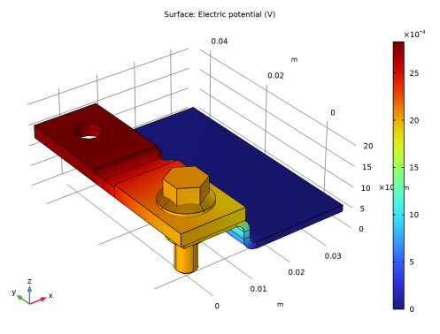
In the Settings window for 3D Plot Group, type Electrode Potential vs. Ground (cd) in the Label text field.
Surface 1
1
In the Electrode Potential vs. Ground (cd) toolbar, click  Surface.
2
In the Settings window for Surface, click Replace Expression in the upper-right corner of the Expression section. From the menu, choose Component 1 (comp1)>Secondary Current Distribution>cd.phis - Electric potential - V.
3
In the Electrode Potential vs. Ground (cd) toolbar, click  Plot.
Electrode Potential vs. Adjacent Reference (cdsh)
1
In the Home toolbar, click  Add Plot Group and choose 3D Plot Group.
2
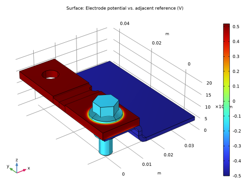
In the Settings window for 3D Plot Group, type Electrode Potential vs. Adjacent Reference (cdsh) in the Label text field.
Surface 1
1
In the Electrode Potential vs. Adjacent Reference (cdsh) toolbar, click  Surface.
2
In the Settings window for Surface, click Replace Expression in the upper-right corner of the Expression section. From the menu, choose Component 1 (comp1)>Current Distribution, Shell>cdsh.Evsref - Electrode potential vs. adjacent reference - V.
3
In the Electrode Potential vs. Adjacent Reference (cdsh) toolbar, click  Plot.
Electrolyte Potential in Film (cdsh)
1
In the Home toolbar, click  Add Plot Group and choose 3D Plot Group.
2
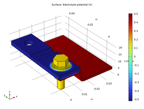
In the Settings window for 3D Plot Group, type Electrolyte Potential in Film (cdsh) in the Label text field.
Surface 1
1
In the Electrolyte Potential in Film (cdsh) toolbar, click  Surface.
2
In the Settings window for Surface, click Replace Expression in the upper-right corner of the Expression section. From the menu, choose Component 1 (comp1)>Current Distribution, Shell>phil2 - Electrolyte potential - V.
3
In the Electrolyte Potential in Film (cdsh) toolbar, click  Plot.
Corrosion Current Density (cdsh)
1
In the Home toolbar, click  Add Plot Group and choose 3D Plot Group.
2
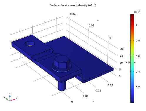
In the Settings window for 3D Plot Group, type Corrosion Current Density (cdsh) in the Label text field.
Surface 1
1
In the Corrosion Current Density (cdsh) toolbar, click  Surface.
2
In the Settings window for Surface, click Replace Expression in the upper-right corner of the Expression section. From the menu, choose Component 1 (comp1)>Current Distribution, Shell>Electrode kinetics>cdsh.iloc_er1 - Local current density - A/m².
3
In the Corrosion Current Density (cdsh) toolbar, click  Plot.
Oxygen Reduction Current Density (cdsh)
1
In the Home toolbar, click  Add Plot Group and choose 3D Plot Group.
2
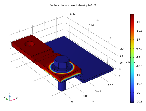
In the Settings window for 3D Plot Group, type Oxygen Reduction Current Density (cdsh) in the Label text field.
Surface 1
1
In the Oxygen Reduction Current Density (cdsh) toolbar, click  Surface.
2
In the Settings window for Surface, click Replace Expression in the upper-right corner of the Expression section. From the menu, choose Component 1 (comp1)>Current Distribution, Shell>Electrode kinetics>cdsh.iloc_er2 - Local current density - A/m².
3
In the Oxygen Reduction Current Density (cdsh) toolbar, click  Plot.