PDF

Atmospheric Corrosion
Introduction
Atmospheric corrosion may occur when thin films of liquid water, in the range of up to hundreds of micrometers, forms on metal surfaces in contact with humidified air. The thickness of the film depends on the relative humidity of the surrounding air, but also on factors such as surface roughness and the presence of particles, especially salt crystals. The thin film of moisture acts as electrolyte, and may cause various corrosion phenomena, such as galvanic corrosion of a bimetallic element or crevice corrosion.
This tutorial model studies atmospheric galvanic corrosion as a function of the relative humidity of the surrounding air and salt load (NaCl) on a bimetallic aluminum alloy – steel surface. It is assumed that the electrolyte film solution is in equilibrium with solid salt particles, distributed uniformly over the surface at a given load.
The example uses parameter data from Ref. 1, Ref. 2, and Ref. 3.
Model Definition
The model set-up is shown in Figure 1.
Figure 1: Model set-up. Each metal surface is 12 mm wide.
The thickness of the electrolyte film depends on both the salt load density and the relative humidity, see Figure 2. The film grows significantly toward 100% relative humidity.
Figure 2: Thickness of the electrolyte for different relative humidities and salt load densities. The conductivity varies linearly with the salt load density. (Ref. 1)
The oxygen solubility, oxygen diffusivity, and the electrolyte conductivity also depend on the relative humidity, see Figure 3, Figure 4, and Figure 5.
Figure 3: Oxygen solubility vs relative humidity.(Ref. 1)
Figure 4: Oxygen diffusivity vs relative humidity.(Ref. 2)
Figure 5: Electrolyte conductivity vs relative humidity. (Ref. 1)
Electrochemical Reactions
The less nobler aluminum alloy is oxidized in the cell, with the electrode reaction kinetics described in terms of experimental polarization data from the corrosion material library.
On the steel surface, oxygen reduction occurs. The oxygen reduction reaction is limited by oxygen transport through the film. The limiting current density, ilim, O2 (SI unit: A/m2), depends on the film thickness, the oxygen solubility and the oxygen diffusivity according to:
where F (96485 C/mol) is Faraday’s constant, D (SI unit: m2/s) is the diffusivity of oxygen in the film, csol (SI unit: mol/m3) is the solubility of oxygen, and dfilm (SI unit: m) is the film thickness.
By assuming a first order dependency of the oxygen reduction kinetics on the local current density of the oxygen concentration, the following expression for the current density, ilim, O2 (SI unit: A/m2), can be derived:
where iexpr is the local current density of the electrode reaction in absence of mass transport limitations described in terms of experimental polarization data from the corrosion material library.
Results and Discussion
Figure 6 shows the local current density of the electrode reactions for a salt load of 0.5 g/m2 and various relative humidities. The cathodic currents reach a plateau close to = 0 at a magnitude that is significantly affected by the relative humidity. This is due to a changing limiting current density for oxygen reduction. As the film thickness grows, the electrolyte transport length for oxygen increases, in combination with an increased oxygen solubility and diffusivity for higher relative humidities.
Figure 6: Local current densities along the metal surface at a salt loading of 0.5 g/m2 and relative humidities (RH) spanning from 80% to 98%.
Figure 7 shows the maximum anodic currents for various salt load densities and relative humidities. For all salt loads, a maximum current density is seen around a relative humidity of 90%.
Figure 7: Maximum metal oxidation anodic current density on the aluminum alloy metal surface for varied relative humidities and salt load densities (LD).
Looking at the maximum cathodic currents in Figure 8, it is seen that the maximum oxygen currents are about one order of magnitude smaller than the anodic currents, but that they follow the same trend with a maximum around a relative humidity of 90%. These currents are very close to the limiting current densities for oxygen reduction.
Figure 8: Maximum oxygen reduction cathodic current densities on the steel metal surface for varied relative humidities and salt load densities (LD).
Finally, Figure 9 shows the average anode current density, which gives us a measure of the total corrosion rate of the sample, for various relative humidities and salt load densities. The maximum is found for a salt load density of 3.5 g/m2 and a relative humidity of 95%.
Figure 9: Average current densities on the aluminum alloy metal surface for varied relative humidities and salt load densities (LD).
Notes About the COMSOL Implementation
The model is implemented using the Current Distribution, Shell interface with two Parametric Sweeps to study the impact of a range of different relative humidities and salt load densities.
References
1. Z.Y. Chen, F. Cui, and R.G. Kelly, “Calculations of the Cathodic Current Delivery Capacity and Stability of Crevice Corrosion under Atmospheric Environments,” J. Electrochemical Society, vol. 155, no. 7, pp. C360–368, 2008.
2. D. Mizuno and R.G. Kelly “Galvanically Induced Intergranular Corrosion of AA5083-H131 Under Atmospheric Exposure Conditions — Part II — Modeling of the Damage Distribution,” Corrosion, vol. 69, no. 6, pp. 580–592, 2013.
3. D. Mizuno, Y. Shi, and R.G. Kelly, “Modeling of Galvanic Interactions between AA5083 and Steel under Atmospheric Conditions,” Excerpt from the Proceedings of the 2011 COMSOL Conference in Boston.
Application Library path: Corrosion_Module/Atmospheric_Corrosion/atmospheric_corrosion
Modeling Instructions
From the File menu, choose New.
New
In the New window, click  Model Wizard.
Model Wizard
1
In the Model Wizard window, click  2D.
2
In the Select Physics tree, select Electrochemistry>Primary and Secondary Current Distribution>Current Distribution, Shell (cdsh).
3
Click Add.
4
Click  Study.
5
In the Select Study tree, select General Studies>Stationary.
6
Geometry 1
Draw the geometry as two adjacent linear polygon segments, each 12 mm wide.
Polygon 1 (pol1)
1
In the Geometry toolbar, click  Polygon.
2
In the Settings window for Polygon, locate the Object Type section.
3
From the Type list, choose Open curve.
4
Locate the Coordinates section. From the Data source list, choose Vectors.
5
In the x text field, type -12[mm] 0 0 12[mm].
6
In the y text field, type 0 0 0 0.
7
Click  Build All Objects.
Global Definitions
Load the model parameters from a text file.
Parameters 1
1
In the Model Builder window, under Global Definitions click Parameters 1.
2
In the Settings window for Parameters, locate the Parameters section.
3
Click  Load from File.
4
Definitions
Now create some average and maximum operators. These will be used later on when postprocessing the simulation results.
Average 1 (aveop1)
1
In the Definitions toolbar, click  Nonlocal Couplings and choose Average.
2
In the Settings window for Average, locate the Source Selection section.
3
From the Geometric entity level list, choose Boundary.
4
Maximum 1 (maxop1)
1
In the Definitions toolbar, click  Nonlocal Couplings and choose Maximum.
2
In the Settings window for Maximum, locate the Source Selection section.
3
From the Geometric entity level list, choose Boundary.
4
Maximum 2 (maxop2)
1
Right-click Maximum 1 (maxop1) and choose Duplicate.
2
In the Settings window for Maximum, locate the Source Selection section.
3
Click  Clear Selection.
4
Materials
Use the Corrosion Material Library to set up the material properties for the electrode kinetics at the aluminum and steel electrode surfaces.
Add Material
1
In the Home toolbar, click  Add Material to open the Add Material window.
2
Go to the Add Material window.
3
In the tree, select Corrosion>Iron Alloys (Steels)>AISI 4340 steel in 0.6M NaCl at pH = 8.3.
4
Click Add to Component in the window toolbar.
Materials
AISI 4340 steel in 0.6M NaCl at pH = 8.3 (mat1)
1
2
In the Model Builder window, expand the AISI 4340 steel in 0.6M NaCl at pH = 8.3 (mat1) node.
Interpolation 1 (iloc_exp)
1
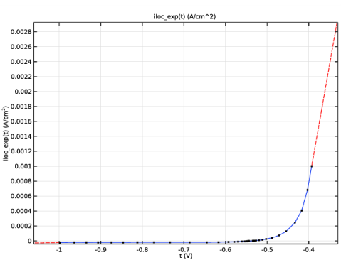
In the Model Builder window, expand the Component 1 (comp1)>Materials>AISI 4340 steel in 0.6M NaCl at pH = 8.3 (mat1)>Local current density (lcd) node, then click Interpolation 1 (iloc_exp).
2
In the Settings window for Interpolation, click  Plot.
The function plot should look like this:
Add Material
1
Go to the Add Material window.
2
In the tree, select Corrosion>Aluminum Alloys>AA5083-H131 in 0.6 M NaCl.
3
Click Add to Component in the window toolbar.
4
In the Home toolbar, click  Add Material to close the Add Material window.
Materials
AA5083-H131 in 0.6 M NaCl (mat2)
1
2
In the Model Builder window, expand the AA5083-H131 in 0.6 M NaCl (mat2) node.
Interpolation 1 (iloc_exp)
1
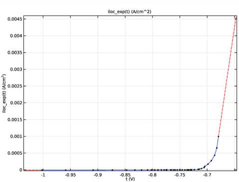
In the Model Builder window, expand the Component 1 (comp1)>Materials>AA5083-H131 in 0.6 M NaCl (mat2)>Local current density (lcd) node, then click Interpolation 1 (iloc_exp).
2
In the Settings window for Interpolation, click  Plot.
The function plot should look like this:
Current Distribution, Shell (cdsh)
Now set up the physics for the current distribution. Start with selecting the reference electrode potential.
1
In the Model Builder window, under Component 1 (comp1) click Current Distribution, Shell (cdsh).
2
In the Settings window for Current Distribution, Shell, click to expand the Physics vs. Materials Reference Electrode Potential section.
3
From the list, choose 0.241 V (SCE vs. SHE).
Electrolyte 1
Next, set the electrolyte thickness and electrolyte conductivity.
1
In the Model Builder window, under Component 1 (comp1)>Current Distribution, Shell (cdsh) click Electrolyte 1.
2
In the Settings window for Electrolyte, locate the Electrolyte section.
3
In the s text field, type d_film.
4
From the σl list, choose User defined. In the associated text field, type sigma.
Electrode Surface 1
Use Electrode Surface nodes to set up the electrode reactions for the two metallic surfaces.
1
In the Physics toolbar, click  Boundaries and choose Electrode Surface.
2
Electrode Reaction 1
1
In the Model Builder window, click Electrode Reaction 1.
2
In the Settings window for Electrode Reaction, locate the Electrode Kinetics section.
3
From the iloc,expr list, choose From material.
Electrode Surface 2
1
In the Physics toolbar, click  Boundaries and choose Electrode Surface.
2
Electrode Reaction 1
1
In the Model Builder window, click Electrode Reaction 1.
2
In the Settings window for Electrode Reaction, locate the Electrode Kinetics section.
3
From the iloc,expr list, choose From material.
4
Select the Limiting current density check box.
5
In the ilim text field, type ilim.
Mesh 1
Use a finer mesh at the intersection point between the two electrode surfaces for this problem.
Edge 1
1
In the Mesh toolbar, click  Edge.
2
Click in the Graphics window and then press Ctrl+A to select both boundaries.
Distribution 1
1
Right-click Edge 1 and choose Distribution.
2
In the Settings window for Distribution, locate the Distribution section.
3
From the Distribution type list, choose Predefined.
4
In the Number of elements text field, type 50.
5
In the Element ratio text field, type 10.
6
Select the Reverse direction check box.
Distribution 2
1
Right-click Distribution 1 and choose Duplicate.
2
3
In the Settings window for Distribution, locate the Distribution section.
4
Clear the Reverse direction check box.
5
Click  Build All.
Your finished mesh should now look like this:
Study 1
The problem is now ready for solving. Use a Parametric Sweep to study the corrosion currents for a range of different relative humidities and salt load densities.
Parametric Sweep
1
In the Study toolbar, click  Parametric Sweep.
2
In the Settings window for Parametric Sweep, locate the Study Settings section.
3
From the Sweep type list, choose All combinations.
4
5
6
7
Solution 1 (sol1)
Decrease the solver tolerance to improve the accuracy of the solutions.
1
In the Study toolbar, click  Show Default Solver.
2
In the Model Builder window, expand the Solution 1 (sol1) node, then click Stationary Solver 1.
3
In the Settings window for Stationary Solver, locate the General section.
4
In the Relative tolerance text field, type 0.00001.
5
In the Study toolbar, click  Compute.
Results
Reproduce the plots from the Results and Discussion section in the following way:
1D Plot Group 5
1
In the Home toolbar, click  Add Plot Group and choose 1D Plot Group.
2
In the Settings window for 1D Plot Group, locate the Axis section.
3
Select the y-axis log scale check box.
Line Graph 1
1
In the 1D Plot Group 5 toolbar, click  Line Graph.
2
In the Settings window for Line Graph, locate the Data section.
3
From the Dataset list, choose Study 1/Solution 1 (sol1).
4
From the Parameter selection (LD) list, choose First.
5
Click in the Graphics window and then press Ctrl+A to select both boundaries.
6
Locate the y-Axis Data section. In the Expression text field, type abs(cdsh.iloc_er1).
7
Select the Description check box. In the associated text field, type Local current density.
8
Locate the x-Axis Data section. From the Parameter list, choose Expression.
9
In the Expression text field, type x.
10
Click to expand the Legends section. Select the Show legends check box.
11
In the 1D Plot Group 5 toolbar, click  Plot.
1D Plot Group 6
In the Home toolbar, click  Add Plot Group and choose 1D Plot Group.
Global 1
1
In the 1D Plot Group 6 toolbar, click  Global.
2
In the Settings window for Global, locate the y-Axis Data section.
3
1D Plot Group 6
1
In the Model Builder window, click 1D Plot Group 6.
2
In the Settings window for 1D Plot Group, click to expand the Title section.
3
From the Title type list, choose Manual.
4
In the Title text area, type Maximum Anode Current Density.
5
Locate the Plot Settings section.
6
Select the x-axis label check box. In the associated text field, type Relative Humidity (1).
7
Select the y-axis label check box. In the associated text field, type Current Density (A/m<sup>2</sup>).
8
Locate the Legend section. From the Position list, choose Upper left.
9
In the 1D Plot Group 6 toolbar, click  Plot.
1D Plot Group 7
Right-click Results>1D Plot Group 6 and choose Duplicate.
Global 1
1
In the Model Builder window, expand the 1D Plot Group 7 node, then click Global 1.
2
In the Settings window for Global, locate the y-Axis Data section.
3
1D Plot Group 7
1
In the Model Builder window, click 1D Plot Group 7.
2
In the Settings window for 1D Plot Group, locate the Title section.
3
In the Title text area, type Maximum Cathode Current Density.
4
In the 1D Plot Group 7 toolbar, click  Plot.
1D Plot Group 8
In the Model Builder window, under Results right-click 1D Plot Group 6 and choose Duplicate.
Global 1
1
In the Model Builder window, expand the 1D Plot Group 8 node, then click Global 1.
2
In the Settings window for Global, locate the y-Axis Data section.
3
1D Plot Group 8
1
In the Model Builder window, click 1D Plot Group 8.
2
In the Settings window for 1D Plot Group, locate the Title section.
3
In the Title text area, type Average Anode Current Density.
4
In the 1D Plot Group 8 toolbar, click  Plot.