
|
|
|
|
{230,15,15} GPa
|
|
|
{15,7,15} GPa
|
|
|
•
|
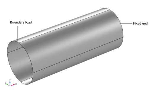
The other end has a transverse load of 50 kN, represented as a uniform boundary load on cross section.
|
|
•
|
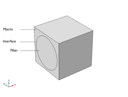
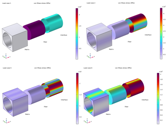
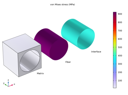
The micromechanics analysis of a single fiber in a bulk matrix with a thin interface between them can be performed using the Cell Periodicity node available in the Solid Mechanics interface. Using this functionality, the elasticity matrix of the homogenized material can be computed for the given fiber, interface, and matrix properties.
|
|
•
|
The Cell Periodicity node has three action buttons in the toolbar of the section called Periodicity Type: Create Load Groups and Study, Create Material by Value, and Create Material by Reference. The action button Create Load Groups and Study generates load groups and a stationary study with load cases. The action button Create Material by Value generates a Global Material with homogenized material properties, with material properties as numbers. The action button Create Material by Reference generates a Global Material with homogenized material properties, with material properties as variables. The action buttons are active depending on the choices in the Periodicity Type and Calculate Average Properties lists.
|
|
•
|
The interface between fiber and matrix can be studied without creating an explicit geometry for the interface using the Thin Layer node available in the Solid Mechanics interface. The solid approximation with a linear elastic material is used to model the thin interface.
|
|
•
|
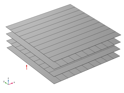
Modeling a composite laminated shell requires a 2D surface geometry, called a base surface, and a Layered Material node that adds an extra dimension (1D) to the base surface geometry in the surface normal direction. Using the Layered Material functionality, you can model several layers of different thicknesses, material properties, and fiber orientations. You can optionally specify the interface materials between the layers and the control mesh elements in each layer.
|
|
•
|
The Layered Material Link and Layered Material Stack have an option to transform the given Layered Material into a symmetric or antisymmetric laminate. A repeated laminate can also be constructed using a transform option.
|
|
•
|
To analyze the results in a composite shell, you can either create a slice plot using the Layered Material Slice plot for in-plane variation of a quantity, or you can create a Through Thickness plot for out-of-plane variation of a quantity at a point. To visualize the results as a 3D solid object, you can use the Layered Material dataset, which creates a virtual 3D solid object combining the surface geometry (2D) and the extra dimension (1D).
|
|
1
|
|
2
|
|
3
|
Click Add.
|
|
4
|
Click
|
|
1
|
|
2
|
|
3
|
|
4
|
Browse to the model’s Application Libraries folder and double-click the file composite_multiscale_parameters.txt.
|
|
1
|
|
2
|
|
3
|
|
4
|
Browse to the model’s Application Libraries folder and double-click the file composite_multiscale_material_properties.txt.
|
|
1
|
|
2
|
|
3
|
|
4
|
Browse to the model’s Application Libraries folder and double-click the file composite_multiscale_strength_properties.txt.
|
|
5
|
In the Model Builder window, right-click Global Definitions and choose Geometry Parts>Part Libraries.
|
|
1
|
In the Part Libraries window, select COMSOL Multiphysics>Representative Volume Elements>3D>unidirectional_fiber_square_packing in the tree.
|
|
2
|
|
3
|
In the Select Part Variant dialog box, select Specify fiber diameter in the Select part variant list.
|
|
4
|
Click OK.
|
|
1
|
|
2
|
In the Settings window for Component, type Component: Micromechanics (Material Properties) in the Label text field.
|
|
1
|
|
2
|
|
4
|
Locate the Position and Orientation of Output section. Find the Displacement subsection. In the xw text field, type -0.005[m].
|
|
5
|
|
6
|
|
1
|
|
2
|
|
3
|
|
1
|
|
2
|
|
3
|
|
4
|
On the object fin, select Boundaries 6–9 only.
|
|
5
|
|
1
|
In the Model Builder window, under Component: Micromechanics (Material Properties) (comp1) right-click Solid Mechanics (solid) and choose Thin Layer.
|
|
2
|
|
3
|
|
4
|
|
1
|
|
2
|
|
3
|
|
4
|
From the Calculate average properties list, choose Elasticity matrix, Standard (XX, YY, ZZ, XY, YZ, XZ).
|
|
1
|
|
2
|
|
3
|
|
1
|
|
2
|
|
3
|
|
1
|
|
2
|
|
3
|
|
1
|
|
2
|
In the Settings window for Cell Periodicity, click Study and Material Generation in the upper-right corner of the Periodicity Type section. From the menu, choose Create Load Groups and Study to generate load groups and a study node.
|
|
1
|
In the Model Builder window, under Component: Micromechanics (Material Properties) (comp1) right-click Materials and choose More Materials>Material Link.
|
|
2
|
|
4
|
|
1
|
|
2
|
|
3
|
|
1
|
In the Model Builder window, under Component: Micromechanics (Material Properties) (comp1)>Solid Mechanics (solid) click Linear Elastic Material 1.
|
|
2
|
|
3
|
|
1
|
In the Model Builder window, under Component: Micromechanics (Material Properties) (comp1) right-click Materials and choose More Materials>Material Link.
|
|
2
|
|
3
|
|
4
|
|
5
|
Click OK.
|
|
6
|
|
7
|
|
1
|
|
2
|
|
3
|
|
1
|
In the Model Builder window, under Component: Micromechanics (Material Properties) (comp1) right-click Materials and choose More Materials>Material Link.
|
|
2
|
|
3
|
Locate the Geometric Entity Selection section. From the Geometric entity level list, choose Boundary.
|
|
4
|
|
5
|
|
1
|
|
2
|
|
3
|
|
1
|
|
2
|
|
3
|
|
4
|
|
1
|
|
2
|
|
3
|
|
4
|
Locate the Destination Boundaries section. From the Selection list, choose Pair 1, Destination (Unidirectional Fiber Composite, Square Packing 1).
|
|
5
|
|
1
|
|
2
|
|
1
|
|
2
|
In the Settings window for Study, type Study: Micromechanics (Material Properties) in the Label text field.
|
|
3
|
|
1
|
|
2
|
|
3
|
|
4
|
|
1
|
|
2
|
|
3
|
|
1
|
|
1
|
In the Model Builder window, under Results>Stress, Unit Cell right-click Volume 1 and choose Duplicate.
|
|
2
|
|
3
|
|
4
|
|
1
|
|
2
|
|
3
|
|
1
|
|
2
|
|
3
|
|
4
|
|
5
|
|
1
|
|
2
|
|
1
|
|
2
|
|
3
|
|
5
|
|
1
|
|
2
|
|
3
|
|
4
|
|
1
|
In the Model Builder window, under Component: Micromechanics (Material Properties) (comp1)>Solid Mechanics (solid) click Cell Periodicity 1.
|
|
2
|
In the Settings window for Cell Periodicity, click Study and Material Generation in the upper-right corner of the Periodicity Type section. From the menu, choose Create Material by Value to generate a global material node with computed elastic properties.
|
|
1
|
|
2
|
|
3
|
|
4
|
|
5
|
|
6
|
|
7
|
|
8
|
|
1
|
In the Model Builder window, expand the Component: Macromechanics (Global Response) (comp2)>Definitions node, then click Boundary System 2 (sys2).
|
|
2
|
|
3
|
|
1
|
|
2
|
|
3
|
|
4
|
Find the Physics interfaces in study subsection. In the table, clear the Solve check box for Study: Micromechanics (Material Properties).
|
|
5
|
|
6
|
|
1
|
In the Model Builder window, under Global Definitions right-click Materials and choose Layered Material.
|
|
2
|
In the Settings window for Layered Material, type Layered Material: [90/0]_2 in the Label text field.
|
|
3
|
|
4
|
Click Add.
|
|
1
|
In the Model Builder window, under Component: Macromechanics (Global Response) (comp2) right-click Materials and choose Layers>Layered Material Link.
|
|
2
|
|
3
|
|
4
|
|
5
|
Click to expand the Preview Plot Settings section. In the Thickness-to-width ratio text field, type 0.4.
|
|
6
|
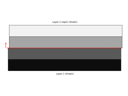
Locate the Layered Material Settings section. Click Layer Cross-Section Preview in the upper-right corner of the section to enable the through-thickness view of the laminated material.
|
|
7
|
Click Layer Stack Preview in the upper-right corner of the Layered Material Settings section to show the stacking sequence including the fiber orientation.
|
|
1
|
In the Model Builder window, under Component: Macromechanics (Global Response) (comp2)>Layered Shell (lshell) click Linear Elastic Material 1.
|
|
2
|
|
3
|
|
1
|
|
2
|
|
3
|
|
1
|
|
2
|
|
3
|
|
4
|
|
5
|
|
1
|
In the Model Builder window, under Global Definitions>Materials click Homogeneous Material (solidcp1mat).
|
|
2
|
|
1
|
|
1
|
|
3
|
|
4
|
|
5
|
|
1
|
|
2
|
|
3
|
|
1
|
|
2
|
|
3
|
|
4
|
|
5
|
|
1
|
|
2
|
|
3
|
|
4
|
Find the Physics interfaces in study subsection. In the table, clear the Solve check box for Solid Mechanics (solid).
|
|
5
|
|
6
|
|
1
|
|
2
|
In the Settings window for Study, type Study: Macromechanics (Global Response) in the Label text field.
|
|
3
|
|
1
|
|
2
|
|
3
|
|
1
|
|
2
|
|
3
|
|
4
|
|
5
|
|
1
|
|
2
|
|
3
|
|
4
|
|
5
|
|
1
|
|
2
|
In the tree, select Study: Macromechanics (Global Response)/Solution 1 (3) (sol1)>Layered Shell>Stress, Slice (lshell).
|
|
3
|
|
4
|
|
1
|
In the Model Builder window, expand the Results>Stress, Slice (lshell) node, then click Stress, Slice (lshell).
|
|
2
|
|
3
|
|
1
|
|
2
|
|
3
|
|
4
|
|
5
|
|
6
|
Locate the Through-Thickness Location section. From the Location definition list, choose Interfaces.
|
|
7
|
|
8
|
|
9
|
|
10
|
|
11
|
|
12
|
|
13
|
|
1
|
|
2
|
|
1
|
|
2
|
|
1
|
|
2
|
|
3
|
|
4
|
|
5
|
Locate the Expressions section. In the table, enter the following settings:
|
|
6
|
|
7
|
Click
|
|
1
|
|
2
|
|
3
|
|
4
|
|
5
|
|
6
|
|
7
|
|
8
|
|
1
|
|
2
|
In the tree, select Study: Macromechanics (Global Response)/Solution 1 (3) (sol1)>Layered Shell>Stress, Through Thickness (lshell).
|
|
3
|
|
4
|
|
1
|
|
2
|
In the Settings window for 1D Plot Group, type von Mises Stress, Through Thickness in the Label text field.
|
|
3
|
|
1
|
In the Model Builder window, expand the von Mises Stress, Through Thickness node, then click Through Thickness 1.
|
|
2
|
|
3
|
|
4
|
|
5
|
|
6
|
|
1
|
|
2
|
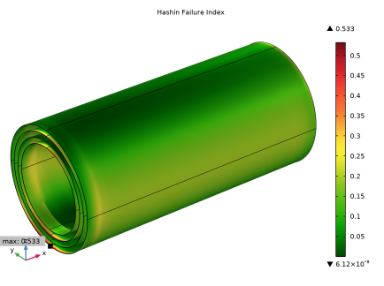
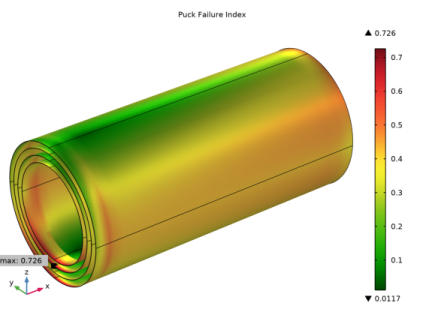
In the tree, select Study: Macromechanics (Global Response)/Solution 1 (3) (sol1)>Layered Shell>Failure Indices (lshell)>Failure Index (Safety 1).
|
|
3
|
|
1
|
|
2
|
|
3
|
|
4
|
|
5
|
|
1
|
|
2
|
|
3
|
|
1
|
|
2
|
|
3
|
|
4
|
|
5
|
|
6
|
|
7
|
|
8
|
|
9
|
|
1
|
|
2
|
In the tree, select Study: Macromechanics (Global Response)/Solution 1 (3) (sol1)>Layered Shell>Failure Indices (lshell)>Failure Index (Safety 2).
|
|
3
|
|
4
|
|
1
|
|
2
|
|
3
|
|
4
|
|
5
|
|
1
|
|
2
|
|
3
|
|
4
|
|
5
|
|
6
|
|
7
|
|
8
|
|
9
|
|
1
|
|
2
|
In the Settings window for Evaluation Group, type Hashin Failure Indexes (Study: Macromechanics (Global Response)) in the Label text field.
|
|
3
|
|
1
|
Right-click Hashin Failure Indexes (Study: Macromechanics (Global Response)) and choose Maximum>Volume Maximum.
|
|
2
|
In the Settings window for Volume Maximum, click Add Expression in the upper-right corner of the Expressions section. From the menu, choose Component: Macromechanics (Global Response) (comp2)>Layered Shell>Safety>Hashin>lshell.lemm1.sf1.f_ifT - Hashin fiber tensile failure index.
|
|
3
|
Click Add Expression in the upper-right corner of the Expressions section. From the menu, choose Component: Macromechanics (Global Response) (comp2)>Layered Shell>Safety>Hashin>lshell.lemm1.sf1.f_ifC - Hashin fiber compressive failure index.
|
|
4
|
Click Add Expression in the upper-right corner of the Expressions section. From the menu, choose Component: Macromechanics (Global Response) (comp2)>Layered Shell>Safety>Hashin>lshell.lemm1.sf1.f_imT - Hashin matrix tensile failure index.
|
|
5
|
Click Add Expression in the upper-right corner of the Expressions section. From the menu, choose Component: Macromechanics (Global Response) (comp2)>Layered Shell>Safety>Hashin>lshell.lemm1.sf1.f_imC - Hashin matrix compressive failure index.
|
|
6
|
Click Add Expression in the upper-right corner of the Expressions section. From the menu, choose Component: Macromechanics (Global Response) (comp2)>Layered Shell>Safety>Hashin>lshell.lemm1.sf1.f_iiT - Hashin interlaminar tensile failure index.
|
|
7
|
Click Add Expression in the upper-right corner of the Expressions section. From the menu, choose Component: Macromechanics (Global Response) (comp2)>Layered Shell>Safety>Hashin>lshell.lemm1.sf1.f_iiC - Hashin interlaminar compressive failure index.
|
|
1
|
In the Model Builder window, click Hashin Failure Indexes (Study: Macromechanics (Global Response)).
|
|
2
|
|
3
|
Select the Transpose check box.
|
|
4
|
|
1
|
|
2
|
In the Settings window for Evaluation Group, type Puck Failure Indexes (Study: Macromechanics (Global Response)) in the Label text field.
|
|
3
|
|
1
|
Right-click Puck Failure Indexes (Study: Macromechanics (Global Response)) and choose Maximum>Volume Maximum.
|
|
2
|
In the Settings window for Volume Maximum, click Add Expression in the upper-right corner of the Expressions section. From the menu, choose Component: Macromechanics (Global Response) (comp2)>Layered Shell>Safety>Puck>lshell.lemm1.sf2.f_ifT - Puck fiber tensile failure index.
|
|
3
|
Click Add Expression in the upper-right corner of the Expressions section. From the menu, choose Component: Macromechanics (Global Response) (comp2)>Layered Shell>Safety>Puck>lshell.lemm1.sf2.f_ifC - Puck fiber compressive failure index.
|
|
4
|
Click Add Expression in the upper-right corner of the Expressions section. From the menu, choose Component: Macromechanics (Global Response) (comp2)>Layered Shell>Safety>Puck>lshell.lemm1.sf2.f_imA - Puck interfiber mode A failure index.
|
|
5
|
Click Add Expression in the upper-right corner of the Expressions section. From the menu, choose Component: Macromechanics (Global Response) (comp2)>Layered Shell>Safety>Puck>lshell.lemm1.sf2.f_imB - Puck interfiber mode B failure index.
|
|
6
|
Click Add Expression in the upper-right corner of the Expressions section. From the menu, choose Component: Macromechanics (Global Response) (comp2)>Layered Shell>Safety>Puck>lshell.lemm1.sf2.f_imC - Puck interfiber mode C failure index.
|
|
1
|
|
2
|
|
3
|
Select the Transpose check box.
|
|
4
|
|
1
|
In the Model Builder window, under Results, Ctrl-click to select Stress (lshell), von Mises Stress, Slice, von Mises Stress, Through Thickness, Hashin Failure Index, and Puck Failure Index.
|
|
2
|
Right-click and choose Group.
|
|
1
|
|
2
|
|
3
|
Locate the Parameters section. In the table, enter the following settings:
|
|
4
|
|
5
|
|
6
|
|
8
|
|
9
|
|
11
|
|
12
|
|
14
|
|
15
|
|
17
|
|
18
|
|
1
|
|
2
|
|
3
|
In the Settings window for Component, type Component: Micromechanics (Local Response) in the Label text field.
|
|
1
|
|
2
|
Select the object pi1 only.
|
|
3
|
|
4
|
|
5
|
|
1
|
|
2
|
|
3
|
|
1
|
|
2
|
|
3
|
Find the Coordinate names subsection. From the Create first tangent direction from list, choose Rotated System 4 (sys4).
|
|
4
|
|
1
|
|
2
|
|
3
|
|
4
|
Browse to the model’s Application Libraries folder and double-click the file composite_multiscale_variables.txt.
|
|
1
|
In the Model Builder window, expand the Component: Micromechanics (Local Response) (comp3)>Solid Mechanics (solid2) node, then click Linear Elastic Material 1.
|
|
2
|
|
3
|
|
1
|
|
2
|
|
4
|
|
5
|
|
6
|
|
1
|
|
2
|
|
4
|
|
5
|
|
6
|
|
1
|
|
2
|
|
3
|
|
4
|
|
5
|
|
1
|
In the Model Builder window, under Component: Micromechanics (Local Response) (comp3)>Solid Mechanics (solid2) click Cell Periodicity 1.
|
|
2
|
|
3
|
From the list, choose Mixed.
|
|
4
|
Find the XX component subsection. In the εavgXX text field, type comp2.at2(X0,Y0,Z0,comp2.lshell.atxd1(xd,comp2.lshell.eXX))*para.
|
|
5
|
Find the YY component subsection. In the εavgYY text field, type comp2.at2(X0,Y0,Z0,comp2.lshell.atxd1(xd,comp2.lshell.eYY))*para.
|
|
6
|
Find the ZZ component subsection. In the εavgZZ text field, type comp2.at2(X0,Y0,Z0,comp2.lshell.atxd1(xd,comp2.lshell.eZZ))*para.
|
|
7
|
Find the XY component subsection. In the εavgXY text field, type comp2.at2(X0,Y0,Z0,comp2.lshell.atxd1(xd,comp2.lshell.eXY))*para.
|
|
8
|
Find the YZ component subsection. In the εavgYZ text field, type comp2.at2(X0,Y0,Z0,comp2.lshell.atxd1(xd,comp2.lshell.eYZ))*para.
|
|
9
|
Find the XZ component subsection. In the εavgXZ text field, type comp2.at2(X0,Y0,Z0,comp2.lshell.atxd1(xd,comp2.lshell.eXZ))*para.
|
|
1
|
In the Model Builder window, expand the Component: Micromechanics (Local Response) (comp3)>Mesh 1 node, then click Free Triangular 1.
|
|
2
|
|
3
|
|
4
|
|
1
|
|
2
|
|
3
|
|
4
|
Locate the Destination Boundaries section. From the Selection list, choose Pair 1, Destination (Unidirectional Fiber Composite, Square Packing 1).
|
|
5
|
|
1
|
|
2
|
|
3
|
|
4
|
Find the Physics interfaces in study subsection. In the table, clear the Solve check boxes for Solid Mechanics (solid) and Layered Shell (lshell).
|
|
5
|
|
6
|
|
1
|
|
2
|
In the Settings window for Study, type Study: Micromechanics (Local Response) in the Label text field.
|
|
3
|
|
1
|
|
2
|
|
3
|
|
4
|
Click
|
|
1
|
|
2
|
|
3
|
Click
|
|
1
|
|
2
|
|
3
|
Find the Values of variables not solved for subsection. From the Settings list, choose User controlled.
|
|
4
|
|
5
|
|
6
|
|
1
|
|
2
|
|
1
|
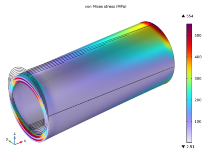
In the Model Builder window, expand the Micromechanics (Local Response) node, then click Stress, Unit Cell 1.
|
|
2
|
In the Settings window for 3D Plot Group, type Stress, Unit Cell (At First Material Point in Inner Layer) in the Label text field.
|
|
3
|
Locate the Data section. From the Dataset list, choose Study: Micromechanics (Local Response)/Parametric Solutions 1 (9) (sol3).
|
|
4
|
|
5
|
|
6
|
|
1
|
In the Model Builder window, expand the Stress, Unit Cell (At First Material Point in Inner Layer) node, then click Volume 1.
|
|
2
|
|
3
|
|
4
|
|
1
|
|
2
|
|
3
|
|
1
|
In the Model Builder window, under Results>Micromechanics (Local Response)>Stress, Unit Cell (At First Material Point in Inner Layer) click Volume 2.
|
|
2
|
|
3
|
|
4
|
|
1
|
|
2
|
|
3
|
|
1
|
In the Model Builder window, under Results>Micromechanics (Local Response)>Stress, Unit Cell (At First Material Point in Inner Layer) click Surface 1.
|
|
2
|
|
3
|
|
4
|
|
1
|
|
2
|
|
3
|
|
5
|
|
6
|
|
1
|
|
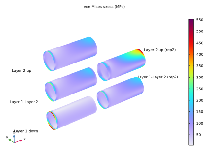
2
|
In the Settings window for 3D Plot Group, type Stress, Unit Cell (At Multiple Material Points) in the Label text field.
|
|
3
|
Locate the Data section. From the Dataset list, choose Study: Micromechanics (Local Response)/Parametric Solutions 1 (9) (sol3).
|
|
4
|
|
5
|
|
6
|
|
7
|
|
1
|
|
2
|
|
3
|
From the Dataset list, choose Study: Micromechanics (Local Response)/Parametric Solutions 1 (9) (sol3).
|
|
4
|
|
5
|
|
6
|
|
7
|
|
8
|
|
9
|
|
10
|
|
11
|
|
12
|
Click OK.
|
|
13
|
|
14
|
|
15
|
|
16
|
|
17
|
|
1
|
|
2
|
|
3
|
|
4
|
|
5
|
|
1
|
In the Model Builder window, under Results>Micromechanics (Local Response)>Stress, Unit Cell (At Multiple Material Points) right-click Surface 1 and choose Duplicate.
|
|
2
|
|
3
|
|
4
|
|
1
|
|
2
|
|
3
|
|
1
|
|
2
|
|
3
|
|
1
|
|
2
|
|
3
|
|
1
|
In the Model Builder window, under Results>Micromechanics (Local Response)>Stress, Unit Cell (At Multiple Material Points) right-click Surface 4 and choose Duplicate.
|
|
2
|
|
3
|
|
1
|
|
2
|
|
3
|
|
1
|
|
2
|
|
3
|
|
4
|
|
1
|
|
2
|
|
3
|
|
1
|
|
2
|
|
3
|
|
1
|
|
2
|
|
3
|
|
1
|
|
2
|
|
3
|
|
1
|
In the Model Builder window, under Results>Micromechanics (Local Response)>Stress, Unit Cell (At Multiple Material Points) right-click Surface 10 and choose Duplicate.
|
|
2
|
|
3
|
|
1
|
|
2
|
|
3
|
|
1
|
In the Model Builder window, right-click Stress, Unit Cell (At Multiple Material Points) and choose Line.
|
|
2
|
|
3
|
|
4
|
|
5
|
|
6
|
|
1
|
|
2
|
|
1
|
In the Model Builder window, right-click Stress, Unit Cell (At First Material Point in Inner Layer) and choose Duplicate.
|
|
2
|
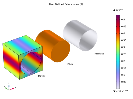
In the Settings window for 3D Plot Group, type User Defined Failure Indexes (At First Material Point in Inner Layer) in the Label text field.
|
|
3
|
|
4
|
|
1
|
In the Model Builder window, expand the User Defined Failure Indexes (At First Material Point in Inner Layer) node, then click Volume 1.
|
|
2
|
In the Settings window for Volume, click Replace Expression in the upper-right corner of the Expression section. From the menu, choose Component: Micromechanics (Local Response) (comp3)>Solid Mechanics>Safety>User defined>solid2.lemm1.sf2.f_i - User-defined failure index.
|
|
1
|
|
2
|
In the Settings window for Volume, click Replace Expression in the upper-right corner of the Expression section. From the menu, choose Component: Micromechanics (Local Response) (comp3)>Solid Mechanics>Safety>User defined>solid2.lemm1.sf1.f_i - User-defined failure index.
|
|
1
|
|
2
|
In the Settings window for Surface, click Replace Expression in the upper-right corner of the Expression section. From the menu, choose Component: Micromechanics (Local Response) (comp3)>Solid Mechanics>Safety>User defined>solid2.tl1.lemm1.sf1.f_i - User-defined failure index.
|
|
1
|
|
2
|
In the Model Builder window, click User Defined Failure Indexes (At First Material Point in Inner Layer).
|
|
3
|
|
1
|
Right-click User Defined Failure Indexes (At First Material Point in Inner Layer) and choose Duplicate.
|
|
2
|
In the Settings window for 3D Plot Group, type User Defined Failure Indexes (At First Material Point in Outer Layer) in the Label text field.
|
|
3
|
|
4
|
|
5
|
|
1
|
|
2
|
In the Settings window for Evaluation Group, type User Defined Failure Indexes at First Material Point in Inner Layer (Study: Micromechanics (Local Response)) in the Label text field.
|
|
3
|
Locate the Data section. From the Dataset list, choose Study: Micromechanics (Local Response)/Parametric Solutions 1 (9) (sol3).
|
|
4
|
|
5
|
|
1
|
Right-click User Defined Failure Indexes at First Material Point in Inner Layer (Study: Micromechanics (Local Response)) and choose Maximum>Volume Maximum.
|
|
3
|
In the Settings window for Volume Maximum, click Replace Expression in the upper-right corner of the Expressions section. From the menu, choose Component: Micromechanics (Local Response) (comp3)>Solid Mechanics>Safety>User defined>solid2.lemm1.sf2.f_i - User-defined failure index.
|
|
4
|
Locate the Expressions section. In the table, enter the following settings:
|
|
1
|
In the Model Builder window, right-click User Defined Failure Indexes at First Material Point in Inner Layer (Study: Micromechanics (Local Response)) and choose Maximum>Volume Maximum.
|
|
3
|
In the Settings window for Volume Maximum, click Replace Expression in the upper-right corner of the Expressions section. From the menu, choose Component: Micromechanics (Local Response) (comp3)>Solid Mechanics>Safety>User defined>solid2.lemm1.sf1.f_i - User-defined failure index.
|
|
4
|
Locate the Expressions section. In the table, enter the following settings:
|
|
1
|
Right-click User Defined Failure Indexes at First Material Point in Inner Layer (Study: Micromechanics (Local Response)) and choose Maximum>Surface Maximum.
|
|
2
|
|
3
|
|
4
|
Click Replace Expression in the upper-right corner of the Expressions section. From the menu, choose Component: Micromechanics (Local Response) (comp3)>Solid Mechanics>Safety>User defined>solid2.tl1.lemm1.sf1.f_i - User-defined failure index.
|
|
5
|
Locate the Expressions section. In the table, enter the following settings:
|
|
1
|
In the Model Builder window, click User Defined Failure Indexes at First Material Point in Inner Layer (Study: Micromechanics (Local Response)).
|
|
2
|
|
3
|
Select the Transpose check box.
|
|
4
|
|
5
|
In the User Defined Failure Indexes at First Material Point in Inner Layer (Study: Micromechanics (Local Response)) toolbar, click
|
|
1
|
Right-click User Defined Failure Indexes at First Material Point in Inner Layer (Study: Micromechanics (Local Response)) and choose Duplicate.
|
|
2
|
In the Settings window for Evaluation Group, type User Defined Failure Indexes at First Material Point in Outer Layer (Study: Micromechanics (Local Response)) in the Label text field.
|
|
3
|
|
4
|
In the User Defined Failure Indexes at First Material Point in Outer Layer (Study: Micromechanics (Local Response)) toolbar, click
|