|
|
|

|
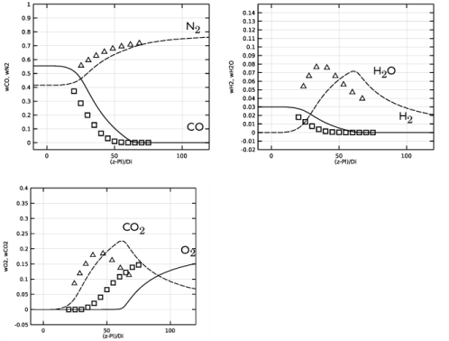
N2
|
||
|
H2
|
||
|
O2
|
||
|
CO2
|
|
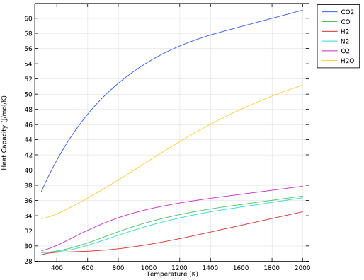
Cp (J/mol/K)
|
Cp (J/mol/K)
|
Cp (J/mol/K)
|
Cp (J/mol/K)
|
|
|
N2
|
||||
|
H2
|
||||
|
O2
|
||||
|
CO2
|
|
1
|
|
2
|
In the Select Physics tree, select Chemical Species Transport>Nonisothermal Reacting Flow>Turbulent Flow>Turbulent Flow, k-ω.
|
|
3
|
Click Add.
|
|
4
|
|
5
|
|
6
|
In the Mass fractions table, enter the following settings:
|
|
7
|
Click
|
|
8
|
|
9
|
Click
|
|
1
|
|
2
|
|
3
|
|
4
|
Browse to the model’s Application Libraries folder and double-click the file round_jet_burner_parameters.txt.
|
|
1
|
|
2
|
|
3
|
|
4
|
|
5
|
|
1
|
|
2
|
|
3
|
|
4
|
|
5
|
|
6
|
|
1
|
|
2
|
On the object r2, select Points 3 and 4 only.
|
|
3
|
|
4
|
|
5
|
|
6
|
|
1
|
|
2
|
|
3
|
|
4
|
|
5
|
|
6
|
|
1
|
|
2
|
|
3
|
|
4
|
|
5
|
|
1
|
|
2
|
Select the object uni1 only.
|
|
3
|
|
4
|
|
5
|
Select the object cha1 only.
|
|
6
|
|
1
|
|
2
|
|
3
|
|
4
|
|
5
|
|
6
|
|
7
|
|
8
|
|
1
|
|
2
|
|
3
|
|
4
|
|
5
|
|
6
|
|
7
|
|
8
|
|
9
|
|
1
|
|
2
|
|
3
|
|
4
|
|
5
|
|
6
|
|
7
|
|
8
|
|
9
|
|
1
|
|
2
|
|
3
|
|
4
|
|
5
|
|
6
|
|
7
|
|
8
|
|
9
|
|
1
|
|
2
|
|
1
|
|
2
|
|
3
|
|
4
|
|
1
|
|
2
|
On the object mce1, select Boundaries 3 and 11 only.
|
|
3
|
|
1
|
|
2
|
Click Next in the window toolbar.
|
|
1
|
|
2
|
|
3
|
|
4
|
|
5
|
|
6
|
|
7
|
|
8
|
|
9
|
|
10
|
|
11
|
|
12
|
|
13
|
|
14
|
Click Next in the window toolbar.
|
|
1
|
|
2
|
Click Finish in the window toolbar.
|
|
1
|
In the Model Builder window, under Global Definitions>Thermodynamics right-click Gas System 1 (pp1) and choose Species Property.
|
|
1
|
|
2
|
|
3
|
|
4
|
|
5
|
|
6
|
Click Next in the window toolbar.
|
|
1
|
|
2
|
Click Next in the window toolbar.
|
|
1
|
|
2
|
|
3
|
Click Next in the window toolbar.
|
|
1
|
|
2
|
Click Finish in the window toolbar.
|
|
1
|
In the Model Builder window, under Component 1 (comp1) right-click Chemistry (chem) and choose Reaction.
|
|
2
|
|
3
|
|
4
|
Click Apply.
|
|
1
|
|
2
|
|
3
|
|
4
|
Click Apply.
|
|
5
|
|
1
|
|
2
|
|
3
|
|
1
|
|
2
|
|
3
|
Select the Thermodynamics check box.
|
|
4
|
Locate the Species Matching section. From the Species solved for list, choose Transport of Concentrated Species.
|
|
5
|
|
6
|
Click to expand the Calculate Transport Properties section. From the Thermal conductivity list, choose User defined.
|
|
7
|
|
8
|
|
9
|
|
1
|
|
3
|
|
4
|
|
5
|
|
6
|
|
7
|
|
8
|
|
9
|
|
1
|
|
2
|
|
3
|
|
4
|
|
5
|
|
6
|
|
1
|
|
2
|
|
3
|
|
4
|
|
5
|
|
1
|
|
2
|
|
3
|
|
4
|
|
5
|
|
1
|
In the Model Builder window, under Component 1 (comp1) click Transport of Concentrated Species (tcs).
|
|
2
|
In the Settings window for Transport of Concentrated Species, locate the Transport Mechanisms section.
|
|
3
|
|
4
|
|
1
|
In the Model Builder window, under Component 1 (comp1)>Transport of Concentrated Species (tcs) click Initial Values 1.
|
|
2
|
|
3
|
|
4
|
|
5
|
|
6
|
|
7
|
|
1
|
|
3
|
|
4
|
|
5
|
|
6
|
|
7
|
|
8
|
|
9
|
|
1
|
|
2
|
|
3
|
|
4
|
|
5
|
|
6
|
|
7
|
|
1
|
|
1
|
In the Model Builder window, under Component 1 (comp1)>Turbulent Flow, k-ω (spf) click Fluid Properties 1.
|
|
2
|
|
3
|
|
4
|
|
5
|
|
1
|
|
3
|
|
4
|
|
5
|
|
1
|
|
3
|
|
4
|
|
5
|
|
6
|
|
7
|
|
8
|
In the text field, type 0.1*Di.
|
|
1
|
|
3
|
|
4
|
|
1
|
In the Model Builder window, under Component 1 (comp1)>Heat Transfer in Fluids (ht) click Initial Values 1.
|
|
2
|
|
3
|
|
1
|
|
2
|
|
3
|
|
4
|
|
5
|
Locate the Heat Conduction, Fluid section. From the k list, choose User defined. In the associated text field, type k_mix.
|
|
6
|
|
7
|
|
1
|
|
3
|
|
4
|
|
1
|
|
1
|
|
2
|
|
3
|
|
1
|
|
3
|
|
4
|
|
5
|
|
6
|
|
7
|
|
1
|
|
3
|
|
4
|
|
5
|
|
6
|
|
7
|
|
1
|
|
3
|
|
4
|
|
5
|
|
6
|
|
7
|
|
8
|
|
1
|
|
3
|
|
4
|
|
5
|
|
6
|
|
7
|
|
8
|
|
1
|
|
3
|
|
4
|
|
5
|
|
6
|
|
7
|
|
1
|
|
3
|
|
4
|
|
5
|
|
6
|
|
7
|
|
8
|
|
9
|
|
1
|
In the Model Builder window, expand the Study 1>Solver Configurations>Solution 1 (sol1)>Stationary Solver 1 node, then click Segregated 1.
|
|
2
|
|
3
|
|
4
|
|
5
|
|
6
|
In the Model Builder window, expand the Study 1>Solver Configurations>Solution 1 (sol1)>Stationary Solver 1>Segregated 1 node, then click Velocity u, Pressure p.
|
|
7
|
|
8
|
|
9
|
In the Add dialog box, in the Variables list, choose Wall temperature, downside (comp1.nirf1.TWall_d), Wall temperature, upside (comp1.nirf1.TWall_u), and Temperature (comp1.T).
|
|
10
|
Click OK.
|
|
11
|
In the Model Builder window, under Study 1>Solver Configurations>Solution 1 (sol1)>Stationary Solver 1>Segregated 1 click Turbulence variables.
|
|
12
|
|
13
|
|
14
|
|
15
|
In the Model Builder window, under Study 1>Solver Configurations>Solution 1 (sol1)>Stationary Solver 1>Segregated 1 right-click Temperature and choose Disable.
|
|
1
|
In the Model Builder window, expand the Global Definitions>Thermodynamics>Gas System 1 (pp1)>Mixture>Vapor node, then click Global Definitions>Thermodynamics>Gas System 1 (pp1)>carbon dioxide>Vapor>Enthalpy of formation 1 (EnthalpyF_carbon_dioxide_Gas12, EnthalpyF_carbon_dioxide_Gas12_Dtemperature, EnthalpyF_carbon_dioxide_Gas12_Dpressure).
|
|
2
|
|
4
|
|
1
|
|
2
|
|
1
|
|
2
|
|
3
|
|
1
|
|
1
|
In the Model Builder window, under Results, Ctrl-click to select 1D Plot Group 2, 1D Plot Group 3, 1D Plot Group 4, 1D Plot Group 5, and 1D Plot Group 6.
|
|
2
|
Right-click and choose Delete.
|
|
1
|
In the Model Builder window, under Global Definitions>Thermodynamics>Gas System 1 (pp1)>carbon dioxide>Vapor click Heat capacity (Cp) 1 (HeatCapacityCp_carbon_dioxide_Gas11, HeatCapacityCp_carbon_dioxide_Gas11_Dtemperature, HeatCapacityCp_carbon_dioxide_Gas11_Dpressure).
|
|
2
|
|
4
|
|
1
|
|
2
|
|
3
|
Repeat creating plots for the functions Heat capacity (Cp) 2 - Heat capacity (Cp) 6 using the same temperature limits.
|
|
1
|
|
2
|
Repeat the drag-dropping of functions 3-6 into the Heat Capacity plot group.
|
|
1
|
In the Model Builder window, under Results, Ctrl-click to select 1D Plot Group 3, 1D Plot Group 4, 1D Plot Group 5, 1D Plot Group 6, and 1D Plot Group 7.
|
|
2
|
Right-click and choose Delete.
|
|
1
|
|
2
|
|
3
|
|
4
|
|
5
|
|
6
|
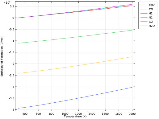
Select the y-axis label check box. In the associated text field, type Enthalpy of Formation (J/mol).
|
|
7
|
|
1
|
|
2
|
|
3
|
|
4
|
|
1
|
|
2
|
|
3
|
|
4
|
|
1
|
|
2
|
|
3
|
|
4
|
|
1
|
|
2
|
|
3
|
|
4
|
|
1
|
|
2
|
|
3
|
|
4
|
|
1
|
|
2
|
|
3
|
|
4
|
|
6
|
|
1
|
|
2
|
|
3
|
|
4
|
|
5
|
|
6
|
|
7
|
|
8
|
|
1
|
|
2
|
|
3
|
|
4
|
|
1
|
|
2
|
|
3
|
|
4
|
|
1
|
|
2
|
|
3
|
|
4
|
|
1
|
|
2
|
|
3
|
|
4
|
|
1
|
|
2
|
|
3
|
|
4
|
|
1
|
|
2
|
|
3
|
|
4
|
|
6
|
|
1
|
|
1
|
|
2
|
|
3
|
Select the Transpose check box.
|
|
1
|
|
2
|
In the Settings window for Global Evaluation, type Enthalpy of Formation, 298 K in the Label text field.
|
|
3
|
Locate the Expressions section. In the table, enter the following settings:
|
|
1
|
|
2
|
|
1
|
|
2
|
|
3
|
Locate the Expressions section. In the table, enter the following settings:
|
|
4
|
|
1
|
|
2
|
|
3
|
Locate the Expressions section. In the table, enter the following settings:
|
|
4
|
|
1
|
In the Model Builder window, under Study 1>Solver Configurations right-click Solution 1 (sol1) and choose Compute.
|
|
2
|
|
1
|
|
2
|
|
3
|
|
4
|
|
5
|
|
6
|
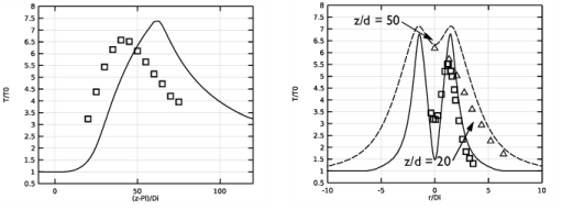
Click to expand the Advanced section. Find the Space variable subsection. In the x text field, type r_mirr20.
|
|
1
|
|
2
|
|
3
|
|
4
|
|
5
|
|
6
|
Locate the Advanced section. Find the Space variable subsection. In the x text field, type r_mirr50.
|
|
1
|
|
2
|
|
3
|
|
4
|
|
1
|
|
2
|
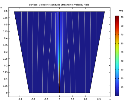
In the Settings window for Streamline, click Replace Expression in the upper-right corner of the Expression section. From the menu, choose Component 1 (comp1)>Heat Transfer in Fluids>Velocity and pressure>ht.ur,ht.uz - Velocity field.
|
|
3
|
|
4
|
|
5
|
Locate the Coloring and Style section. Find the Point style subsection. From the Color list, choose Gray.
|
|
6
|
|
7
|
|
1
|
|
2
|
|
3
|
|
4
|
|
1
|
|
2
|
|
3
|
|
4
|
|
1
|
|
2
|
|
3
|
|
4
|
|
1
|
|
2
|
|
3
|
|
4
|
|
5
|
|
1
|
|
2
|
|
3
|
|
1
|
|
2
|
|
3
|
|
4
|
Browse to the model’s Application Libraries folder and double-click the file round_jet_burner_chnAclY.fav.
|
|
1
|
|
2
|
|
3
|
|
4
|
Browse to the model’s Application Libraries folder and double-click the file round_jet_burner_chnAd20Y.fav.
|
|
1
|
|
2
|
|
3
|
|
4
|
Browse to the model’s Application Libraries folder and double-click the file round_jet_burner_chnAd50Y.fav.
|
|
1
|
|
2
|
|
3
|
|
4
|
Browse to the model’s Application Libraries folder and double-click the file round_jet_burner_seq1420.dat.
|
|
1
|
|
2
|
|
3
|
|
4
|
Browse to the model’s Application Libraries folder and double-click the file round_jet_burner_seq1450.dat.
|
|
1
|
|
3
|
|
4
|
|
5
|
|
6
|
|
7
|
|
8
|
|
9
|
|
1
|
|
2
|
|
3
|
|
4
|
|
5
|
|
6
|
Click to expand the Preprocessing section. Find the x-axis column subsection. From the Preprocessing list, choose Linear.
|
|
7
|
|
8
|
|
9
|
|
10
|
Locate the Coloring and Style section. Find the Line style subsection. From the Line list, choose None.
|
|
11
|
|
12
|
|
13
|
|
14
|
|
1
|
|
2
|
|
3
|
|
4
|
|
5
|
|
6
|
|
7
|
|
8
|
|
9
|
|
10
|
|
11
|
|
12
|
|
13
|
|
14
|
|
1
|
|
2
|
|
3
|
|
1
|
|
2
|
|
3
|
|
4
|
|
5
|
|
6
|
|
7
|
|
8
|
|
9
|
|
1
|
|
2
|
|
3
|
|
4
|
|
5
|
Locate the Coloring and Style section. Find the Line style subsection. From the Line list, choose Dashed.
|
|
6
|
Locate the Legends section. In the table, enter the following settings:
|
|
7
|
|
1
|
|
2
|
|
3
|
|
4
|
|
5
|
|
6
|
|
7
|
Locate the Preprocessing section. Find the x-axis column subsection. From the Preprocessing list, choose Linear.
|
|
8
|
|
9
|
|
10
|
|
11
|
Locate the Coloring and Style section. Find the Line style subsection. From the Line list, choose None.
|
|
12
|
|
13
|
|
14
|
|
15
|
|
1
|
|
2
|
|
3
|
|
4
|
Locate the Coloring and Style section. Find the Line markers subsection. From the Marker list, choose Triangle.
|
|
5
|
|
6
|
Locate the Legends section. In the table, enter the following settings:
|
|
1
|
|
2
|
|
3
|
|
4
|
|
5
|
|
6
|
|
7
|
|
8
|
|
9
|
|
10
|
|
11
|
|
12
|
|
13
|
|
14
|
|
1
|
|
2
|
|
1
|
|
2
|
|
3
|
|
1
|
|
2
|
|
3
|
|
1
|
|
2
|
|
3
|
|
4
|
|
5
|
|
6
|
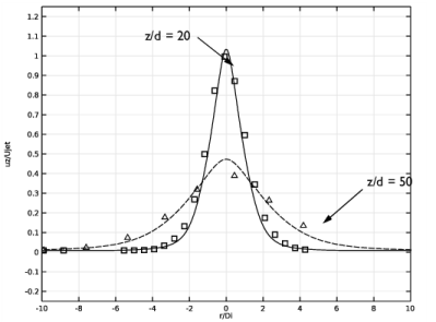
Locate the Preprocessing section. Find the y-axis columns subsection. In the Scaling text field, type 1/Ujet.
|
|
1
|
|
2
|
|
3
|
|
4
|
|
5
|
|
6
|
Locate the Preprocessing section. Find the y-axis columns subsection. In the Scaling text field, type 1/Ujet.
|
|
1
|
|
2
|
|
3
|
|
4
|
|
5
|
|
6
|
|
7
|
|
8
|
|
1
|
|
2
|
|
3
|
|
4
|
|
5
|
|
6
|
|
7
|
|
1
|
|
2
|
|
3
|
|
4
|
Locate the Legends section. In the table, enter the following settings:
|
|
1
|
|
2
|
|
3
|
|
4
|
Locate the Preprocessing section. Find the y-axis columns subsection. In the Scaling text field, type 1.
|
|
5
|
Locate the Legends section. In the table, enter the following settings:
|
|
6
|
|
1
|
In the Model Builder window, under Results>CO, N2 @ centerline right-click Line Graph 1 and choose Duplicate.
|
|
2
|
|
3
|
|
4
|
Locate the Coloring and Style section. Find the Line style subsection. From the Line list, choose Dashed.
|
|
5
|
Locate the Legends section. In the table, enter the following settings:
|
|
1
|
In the Model Builder window, under Results>CO, N2 @ centerline right-click Table Graph 1 and choose Duplicate.
|
|
2
|
|
3
|
|
4
|
Locate the Coloring and Style section. Find the Line markers subsection. From the Marker list, choose Triangle.
|
|
5
|
|
6
|
Locate the Legends section. In the table, enter the following settings:
|
|
7
|
|
1
|
|
2
|
|
3
|
|
4
|
|
1
|
|
2
|
|
3
|
|
4
|
Locate the Legends section. In the table, enter the following settings:
|
|
1
|
|
2
|
|
3
|
|
4
|
Locate the Legends section. In the table, enter the following settings:
|
|
1
|
|
2
|
|
3
|
|
4
|
Locate the Legends section. In the table, enter the following settings:
|
|
1
|
|
2
|
|
3
|
|
4
|
Locate the Legends section. In the table, enter the following settings:
|
|
1
|
|
2
|
|
3
|
|
4
|
|
5
|
|
6
|
|
1
|
|
2
|
|
3
|
|
4
|
|
1
|
|
2
|
|
3
|
|
4
|
Locate the Legends section. In the table, enter the following settings:
|
|
1
|
|
2
|
|
3
|
|
4
|
Locate the Legends section. In the table, enter the following settings:
|
|
1
|
|
2
|
|
3
|
|
4
|
Locate the Legends section. In the table, enter the following settings:
|
|
1
|
|
2
|
|
3
|
|
4
|
Locate the Legends section. In the table, enter the following settings:
|
|
1
|
|
2
|
|
3
|
|
4
|
|
5
|
|
6
|