PDF

Journal Bearing with Cavitation
Introduction
Journal bearings are used to carry radial loads to, for example, support a rotating shaft.
A simple journal bearing consists of two rigid cylinders. The outer cylinder (bearing) wraps the inner rotating journal (shaft). Normally, the position of the journal center is eccentric with the bearing center. A lubricant fills the small annular gap or clearance between the journal and the bearing. The amount of eccentricity of the journal is related to the pressure that is generated in the bearing to balance the radial load. The lubricant is supplied through a hole or a groove and may or may not extend all around the journal.
If the bearing is not designed correctly, the gases dissolved in the lubricant can cause cavitation in the diverging clearance between the journal and the bearing. This happens because the pressure in the lubricant drops below the saturation pressure for the release of dissolved gases. The saturation pressure is normally similar to the ambient pressure. Cavitation can cause damage to the bearing components leading to premature failure.
The following model predicts the onset and extent of cavitation in the lubrication layer. The onset and extent of gaseous cavitation in a journal bearing determine the load that can be applied to the bearing.
This example is based on the Journal Bearing model, that does not include cavitation effects; review that model before beginning this one.
Model Definition
The governing equation, geometry and boundary conditions are discussed for the Journal Bearing model.
With the cavitation feature enabled, the flow in the journal bearing is divided in two regions:
Elrod and Adams derived a general form of the Reynolds equation by introducing a switch function, g, equal to 1 in the full film region (θ  1) and 0 in the cavitation region (θ < 1). This switch function allows for solving a single equation for both the full film and the cavitation region and leads to a modified version of the average velocity used in the Reynold’s equation:
where the first and second terms on the right-hand side correspond to the average Couette and average Poiseuille velocities, respectively. This switch function sets the average Poiseuille velocity is to zero in the cavitation region.
Because the average Poiseuille velocity is set to zero in the cavitation region, the density needs to be a function of the pressure variable and could be defined as
A density that is not pressure dependent would lead to empty equations in the cavitation region since the pressure variable p would no longer be present in the governing equations.
Results and Discussion
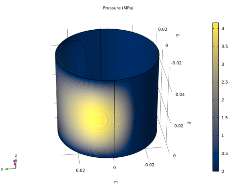
While the pressure is constant and equal to the cavitation pressure in the cavitation region, the computed pressure, pfilm, is negative in this region. The value of this negative pressure can be used to derive the volume fraction of fluid in the cavitation region. The actual or physical pressure, available in the postprocessing section as tff.p, is equal to the computed pressure in the full film region and equal to the cavitation pressure in the cavitation region. Figure 1 shows this physical pressure, tff.p. The maximum pressure is reached in a region closer to the minimum lubricant thickness.
Figure 1: Pressure distribution and pressure contours on the journal.
Figure 2 shows the fluid mass fraction. The mass fraction is equal to 1 in the full film region and less than 1 in the cavitation region (where only part of the volume is occupied by the fluid). It is computed as the minimum value between 1 and the ratio ρ/ρcav, where ρ and ρcav represent the fluid density and the density at the cavitation pressure, respectively.
Figure 2: Fluid mass fraction.
Application Library path: CFD_Module/Thin-Film_Flow/journal_bearing_cavitation
Modeling Instructions
From the File menu, choose New.
New
In the New window, click  Model Wizard.
Model Wizard
1
In the Model Wizard window, click  3D.
2
In the Select Physics tree, select Fluid Flow>Thin-Film Flow>Thin-Film Flow (tff).
3
Click Add.
4
Click  Study.
5
In the Select Study tree, select General Studies>Stationary.
6
Global Definitions
Parameters 1
1
In the Model Builder window, under Global Definitions click Parameters 1.
2
In the Settings window for Parameters, locate the Parameters section.
3
Geometry 1
Cylinder 1 (cyl1)
1
In the Geometry toolbar, click  Cylinder.
2
In the Settings window for Cylinder, locate the Object Type section.
3
From the Type list, choose Surface.
4
Locate the Size and Shape section. In the Radius text field, type R.
5
In the Height text field, type H.
6
Click  Build All Objects.
Definitions
Variables 1
1
In the Home toolbar, click  Variables and choose Local Variables.
2
In the Settings window for Variables, locate the Variables section.
3
Thin-Film Flow (tff)
1
Click the  Show More Options button in the Model Builder toolbar.
2
In the Show More Options dialog box, in the tree, select the check box for the node Physics>Advanced Physics Options.
3
4
In the Model Builder window, under Component 1 (comp1) click Thin-Film Flow (tff).
5
In the Settings window for Thin-Film Flow, locate the Physical Model section.
6
From the Fluid type list, choose Liquid with cavitation.
Fluid-Film Properties 1
1
In the Model Builder window, under Component 1 (comp1)>Thin-Film Flow (tff) click Fluid-Film Properties 1.
2
In the Settings window for Fluid-Film Properties, locate the Fluid Properties section.
3
From the μ list, choose User defined. In the associated text field, type 0.01[Pa*s].
4
Locate the Wall Properties section. In the hw1 text field, type th.
5
Locate the Base Properties section. From the vb list, choose User defined. Specify the vector as
Mesh 1
In the Model Builder window, under Component 1 (comp1) right-click Mesh 1 and choose Build All.
Study 1
In the Home toolbar, click  Compute.
Results
Fluid Pressure (tff)
The default plot group shows the pressure field as a surface plot. Add a contour plot of the same quantity to reproduce the plot in Figure 1.
Surface 1
1
In the Model Builder window, expand the Fluid Pressure (tff) node, then click Surface 1.
2
In the Settings window for Surface, locate the Expression section.
3
In the Expression text field, type tff.p.
4
From the Unit list, choose MPa.
5
Locate the Coloring and Style section. Click  Change Color Table.
6
In the Color Table dialog box, select Linear>Cividis in the tree.
7
Surface 1
1
In the Model Builder window, click Surface 1.
2
In the Fluid Pressure (tff) toolbar, click  Plot.
Contour 1
1
In the Model Builder window, right-click Fluid Pressure (tff) and choose Contour.
2
In the Settings window for Contour, locate the Expression section.
3
In the Expression text field, type tff.p.
4
From the Unit list, choose MPa.
5
Locate the Coloring and Style section. Click  Change Color Table.
6
In the Color Table dialog box, select Linear>GrayScale in the tree.
7
8
In the Settings window for Contour, locate the Coloring and Style section.
9
Clear the Color legend check box.
Fluid Pressure (tff)
1
In the Model Builder window, click Fluid Pressure (tff).
2
In the Settings window for 3D Plot Group, click to expand the Title section.
3
From the Title type list, choose Manual.
4
In the Title text area, type Pressure (MPa).
5
In the Fluid Pressure (tff) toolbar, click  Plot.
6
Click the  Zoom Extents button in the Graphics toolbar.
To see the bearing from different angles just click and drag in the Graphics window.
Mass Fraction
Reproduce Figure 2 by the following these steps.
1
In the Home toolbar, click  Add Plot Group and choose 3D Plot Group.
2
In the Settings window for 3D Plot Group, type Mass Fraction in the Label text field.
Surface 1
1
In the Mass Fraction toolbar, click  Surface.
2
In the Settings window for Surface, click Replace Expression in the upper-right corner of the Expression section. From the menu, choose Component 1 (comp1)>Thin-Film Flow>Cavitation>tff.theta - Mass fraction.
3
In the Mass Fraction toolbar, click  Plot.