PDF

Journal Bearing
Introduction
Journal bearings are used to carry radial loads, for example, to support a rotating shaft.
A simple journal bearing consists of two rigid cylinders. The outer cylinder (bearing) wraps the inner rotating journal (shaft). Normally, the position of the journal center is eccentric with the bearing center. A lubricant fills the small annular gap or clearance between the journal and the bearing. The amount of eccentricity of the journal is related to the pressure that is generated in the bearing to balance the radial load. The lubricant is supplied through a hole or a groove and may or may not extend all around the journal.
Under normal operating conditions, the gases dissolved in the lubricant cause cavitation in the diverging clearance between the journal and the bearing. This happens because the pressure in the lubricant drops below the saturation pressure for the release of dissolved gases. The saturation pressure is normally similar to the ambient pressure. The following model does not account for cavitation and therefore predicts sub-ambient pressures. Such sub-ambient pressures are the result of the so-called Sommerfeld boundary condition. For practical purposes, these sub-ambient pressures should be neglected.
Model Definition
The pressure in the lubricant (SAE 10 at 70° C) is governed by the Reynolds equation. For an incompressible fluid with no slip condition, the stationary Reynolds equation in the continuum range is given by
In this equation, ρ is the density (SI unit: kg/m3), h is the lubricant thickness (SI unit: m), μ is the viscosity (SI unit: Pa·s), p is the pressure (SI unit: Pa), a is the location (m) of the channel base, va is the tangential velocity (SI unit: m/s) of the channel base, b is the location (SI unit: m) of the solid wall, and vb is the tangential velocity (SI unit: m/s) of the solid wall.
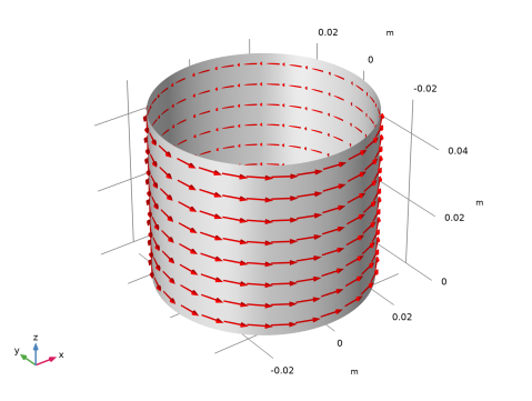
The rotating journal is considered to be the solid wall. Figure 1 shows the rotating journal wall on which you solve the Reynolds equation. Because the pressure is constant through the lubricant film thickness, COMSOL uses the tangential projection of the gradient operator, , to calculate the pressure distribution on the lubricant surface. Note that in this case the term equates to 0, so the governing equation simplifies to
The lubricant thickness, h, is defined as
where c ≡ RB − RJ is the difference between the bearing radius and the journal radius, ε is the eccentricity, and θ is the polar angular coordinate of a point on the lubricant. Figure 2 shows the converging and diverging lubricant thickness around the journal.
Figure 1: Geometry (cylindrical journal) showing the base velocity direction with red arrows.
Figure 2: The lubricant thickness around the rotating journal.
Border Conditions
The pressure at the ends of the cylindrical journal is assumed to be similar to the ambient pressure. Therefore, the border conditions are
where L is the length of the cylindrical journal.
Results and Discussion
Figure 3 shows the calculated pressure distribution and pressure contours. As expected, the maximum pressure is reached in a region closer to the minimum lubricant thickness. Sub-ambient or negative pressure also results due to approximate boundary conditions. For a more accurate modeling of pressure distribution, gaseous cavitation has to be taken into account.
Figure 3: Pressure distribution and pressure contours on the journal.
Application Library path: CFD_Module/Thin-Film_Flow/journal_bearing
Modeling Instructions
From the File menu, choose New.
New
In the New window, click  Model Wizard.
Model Wizard
1
In the Model Wizard window, click  3D.
2
In the Select Physics tree, select Fluid Flow>Thin-Film Flow>Thin-Film Flow (tff).
3
Click Add.
4
Click  Study.
5
In the Select Study tree, select General Studies>Stationary.
6
Global Definitions
Parameters 1
1
In the Model Builder window, under Global Definitions click Parameters 1.
2
In the Settings window for Parameters, locate the Parameters section.
3
Geometry 1
Cylinder 1 (cyl1)
1
In the Geometry toolbar, click  Cylinder.
2
In the Settings window for Cylinder, locate the Object Type section.
3
From the Type list, choose Surface.
4
Locate the Size and Shape section. In the Radius text field, type R.
5
In the Height text field, type H.
6
Click  Build All Objects.
Definitions
Variables 1
1
In the Home toolbar, click  Variables and choose Local Variables.
2
In the Settings window for Variables, locate the Variables section.
3
Thin-Film Flow (tff)
Fluid-Film Properties 1
1
In the Model Builder window, under Component 1 (comp1)>Thin-Film Flow (tff) click Fluid-Film Properties 1.
2
In the Settings window for Fluid-Film Properties, locate the Fluid Properties section.
3
From the ρ list, choose User defined. In the associated text field, type 860[kg/m^3].
4
From the μ list, choose User defined. In the associated text field, type 0.01[Pa*s].
5
Locate the Wall Properties section. In the hw1 text field, type th.
6
Locate the Base Properties section. From the vb list, choose User defined. Specify the vector as
Border 1
As you can see in the Border Settings section, the default condition that applies at the cylinder ends is Zero pressure.
Study 1
In the Home toolbar, click  Compute.
Results
Fluid Pressure (tff)
The default plot group shows the pressure field as a surface plot. Add a contour plot of the same quantity to reproduce the plot in Figure 3.
Surface 1
1
In the Model Builder window, expand the Fluid Pressure (tff) node, then click Surface 1.
2
In the Settings window for Surface, locate the Expression section.
3
From the Unit list, choose MPa.
4
Locate the Coloring and Style section. Click  Change Color Table.
5
In the Color Table dialog box, select Linear>Cividis in the tree.
6
7
In the Settings window for Surface, locate the Coloring and Style section.
8
From the Color table transformation list, choose Reverse.
Contour 1
1
In the Model Builder window, right-click Fluid Pressure (tff) and choose Contour.
2
In the Settings window for Contour, locate the Expression section.
3
From the Unit list, choose MPa.
4
Locate the Coloring and Style section. Click  Change Color Table.
5
In the Color Table dialog box, select Linear>GrayScale in the tree.
6
7
In the Settings window for Contour, locate the Coloring and Style section.
8
Clear the Color legend check box.
Fluid Pressure (tff)
1
In the Model Builder window, click Fluid Pressure (tff).
2
In the Settings window for 3D Plot Group, click to expand the Title section.
3
From the Title type list, choose Manual.
4
In the Title text area, type Pressure (MPa).
5
In the Fluid Pressure (tff) toolbar, click  Plot.
To see the bearing from different angles just click and drag in the Graphics window.
The following steps reproduce Figure 1.
Velocity direction
1
In the Home toolbar, click  Add Plot Group and choose 3D Plot Group.
2
In the Settings window for 3D Plot Group, type Velocity direction in the Label text field.
Surface 1
1
Right-click Velocity direction and choose Surface.
2
In the Settings window for Surface, locate the Coloring and Style section.
3
From the Coloring list, choose Uniform.
4
From the Color list, choose Gray.
Arrow Surface 1
1
In the Model Builder window, right-click Velocity direction and choose Arrow Surface.
2
In the Settings window for Arrow Surface, click Replace Expression in the upper-right corner of the Expression section. From the menu, choose Component 1 (comp1)>Thin-Film Flow>Wall and base properties>tff.vbx,tff.vby,tff.vbz - Velocity of base.
Velocity direction
1
In the Model Builder window, click Velocity direction.
2
In the Settings window for 3D Plot Group, locate the Plot Settings section.
3
Clear the Plot dataset edges check box.
4
Locate the Title section. From the Title type list, choose None.
Reproduce Figure 2 by the following steps.
Lubricant thickness
1
In the Home toolbar, click  Add Plot Group and choose 3D Plot Group.
2
In the Settings window for 3D Plot Group, type Lubricant thickness in the Label text field.
Surface 1
1
Right-click Lubricant thickness and choose Surface.
2
In the Settings window for Surface, click Replace Expression in the upper-right corner of the Expression section. From the menu, choose Component 1 (comp1)>Thin-Film Flow>Wall and base properties>tff.h - Total gap height - m.
3
Locate the Expression section. From the Unit list, choose µm.
4
Locate the Coloring and Style section. Click  Change Color Table.
5
In the Color Table dialog box, select Linear>Cividis in the tree.
6
Surface 1
1
In the Model Builder window, click Surface 1.
2
In the Lubricant thickness toolbar, click  Plot.
Lubricant thickness
1
In the Model Builder window, click Lubricant thickness.
2
In the Settings window for 3D Plot Group, locate the Color Legend section.
3
Select the Show maximum and minimum values check box.