PDF

Thermal Runaway Propagation in a Battery Pack
Introduction
Due to abuse, such as internal or external short circuits or excessive heating, an individual battery cell may go into thermal runaway, during which the battery cell generates a significant amount of heat. If enough heat is transferred between adjacent cells during a thermal runaway event, neighboring cells will also go into thermal runaway.
A thermal runaway propagating through the whole pack constitutes a severe safety hazard. When designing a battery pack, measures need to be taken in order to mitigate runaway propagation.
This tutorial simulates the heat transfer and resulting thermal runaway propagation in a pack consisting of 20 cylindrical cells using event-based heat sources.
For a general introduction to the battery pack interface, the user is also referred to the tutorial Thermal Distribution in a Pack of Cylindrical Batteries.
Model Definition
Figure 1 shows the model geometry. The pack consists of 20 cylindrical batteries in a 5s4p configuration (that is: 5 serial strings of 4 batteries coupled in parallel). Two plastic holder frames are used for fixating the battery locations and cell-to-cell distances. Serial connectors are welded to the battery terminals, and parallel connectors are in turn welded to the serial connectors, midway between the battery cylinders. A thin plastic wrapping encloses the whole pack, thereby forming a compartment of quiescent air surrounding the battery cylinders.
The following materials are used from the built-in material library:
The battery pack model is setup in a similar manner as in the Thermal Distribution in a Pack of Cylindrical Batteries tutorial, using the Battery Pack interface together with a Heat Transfer interface and an Electrochemical Heating multiphysics node. The Battery Layers node in heat transfer is used to define the anisotropic properties of the batter cylinders.
The pack is charged from an initial state of charge of 25% at a 2C rate. The Charge-Discharge Cycling node is used to control the load current so that it is turned of when the pack voltage exceeds 21 V. The initial pack temperature is set to equal the surrounding temperature of 30°C.
Figure 1: Model geometry.
The cell thermal runaway is modeled by the use of Thermal Event nodes in the battery pack interface. At the triggering of a thermal event in a battery cylinder, a time-dependent heat source is released as shown in Figure 2 with a a total released heat equal to 22 kJ. The heat profile was taken from Ref. 1. Due to the loss of electrolyte and the resulting increase of the internal battery resistances, the ohmic resistance of the corresponding battery model in each cylinder is increased about two orders of magnitude when a thermal event is triggered.
To initiate the propagation of the thermal runaway, one cell is assumed to be start malfunctioning at an early stage in the charge cycle (due to an internal short circuit, or similar). The triggering of the malfunctioning cell is set explicitly to begin at t = 1 min into the simulation. For the remaining cells, the thermal events are set to be triggered when the maximum temperature of an individual cell exceeds 80°C.
Figure 2: Heat source released in an individual battery cell when a thermal event is triggered.
Results and Discussion
Figure 3 shows the pack voltage and maximum battery temperature in the pack vs time. The steep gradients in the temperature curve indicate the triggering of the thermal events. At the triggering of each event, a small shift in the pack voltage curve can also be seen, which is related to the corresponding increase in cell resistance, impacting the current distribution in the pack.
During the first minute, only a small temperature increase can be observed. This is due to Joule heating and other processes during normal charging operation. After triggering of the first cell runaway at 1 min, there is a steep increase in the maximum temperature, after which there is an incubation time of several minutes until enough heat has spread to a neighboring cell in order to trigger consecutive runaways. After triggering of this second runaway, the intervals between successive cell runaways become shorter.
After about 10 min, the maximum charging voltage limit has been reached, and the charging of the pack is turned off. However, the thermal runaway continues to propagate through the pack also after this.
A few minutes later, all cells have gone through thermal runaway, and the maximum temperature slowly starts to relax towards the surrounding temperature of 30°C.
Figure 3: Pack voltage and maximum battery temperature in the pack.
The temperature in the pack, excluding the air domain, at various times is shown in Figure 4.
Figure 4: Temperature surface plots at various times.
Reference
1. P.T. Coman, E.C. Darcy, and R.E. White, “Simplified Thermal Runaway Model for Assisting the Design of a Novel Safe Li-Ion Battery Pack,” J. Electrochem. Soc., vol. 169, p. 040516, 2022.
Application Library path: Battery_Design_Module/Thermal_Management/thermal_runaway_propagation
Modeling Instructions
From the File menu, choose New.
New
In the New window, click  Model Wizard.
Model Wizard
1
In the Model Wizard window, click  3D.
2
In the Select Physics tree, select Electrochemistry>Batteries>Battery Pack (bp).
3
Click Add.
4
In the Select Physics tree, select Heat Transfer>Heat Transfer in Solids (ht).
5
Click Add.
6
Click  Study.
7
In the Select Study tree, select General Studies>Time Dependent.
8
Geometry 1
Import the geometry sequence from a file.
1
In the Geometry toolbar, click Insert Sequence and choose Insert Sequence.
2
3
In the Insert Sequence dialog box, select Geometry 1 in the Select geometry sequence to insert list.
4
5
In the Geometry toolbar, click  Build All.
Inspect the imported geometry. You may enable and disable wire frame rendering and transparency to view internal geometry features.
6
Click the  Wireframe Rendering button in the Graphics toolbar.
7
Click the  Wireframe Rendering button in the Graphics toolbar.
8
Click the  Transparency button in the Graphics toolbar.
Geometry 1
In the Model Builder window, collapse the Component 1 (comp1)>Geometry 1 node.
Global Definitions
Geometry Parameters
Some geometry parameters were imported together with the geometry sequence.
1
In the Model Builder window, under Global Definitions click Parameters 1.
2
In the Settings window for Parameters, type Geometry Parameters in the Label text field.
Physics Parameters
Import some additional parameters needed for setting up the physics.
1
In the Home toolbar, click  Parameters and choose Add>Parameters.
2
In the Settings window for Parameters, type Physics Parameters in the Label text field.
3
Locate the Parameters section. Click  Load from File.
4
Add Material
1
In the Home toolbar, click  Add Material to open the Add Material window.
2
Go to the Add Material window.
Add some materials from the built-in material library.
3
4
Right-click and choose Add to Component 1 (comp1).
5
In the tree, select Built-in>Acrylic plastic.
6
Right-click and choose Add to Component 1 (comp1).
7
In the tree, select Built-in>Steel AISI 4340.
8
Right-click and choose Add to Component 1 (comp1).
9
In the Home toolbar, click  Add Material to close the Add Material window.
Materials
Air (mat1)
1
In the Settings window for Material, locate the Geometric Entity Selection section.
2
From the Selection list, choose Air Compartment.
Acrylic plastic (mat2)
1
In the Model Builder window, click Acrylic plastic (mat2).
2
In the Settings window for Material, locate the Geometric Entity Selection section.
3
From the Selection list, choose Holders (Part 3 - Holders 1).
Steel AISI 4340 (mat3)
1
In the Model Builder window, click Steel AISI 4340 (mat3).
2
In the Settings window for Material, locate the Geometric Entity Selection section.
3
From the Selection list, choose All Conductors (Part 2 - Conductors 1).
Battery Pack (bp)
The battery pack interface is active on the battery and conductor domains only.
1
In the Model Builder window, under Component 1 (comp1) click Battery Pack (bp).
2
In the Settings window for Battery Pack, locate the Domain Selection section.
3
From the Selection list, choose Batteries and Conductors.
Batteries
1
In the Model Builder window, under Component 1 (comp1)>Battery Pack (bp) click Batteries.
2
In the Settings window for Batteries, locate the Domain Selection section.
3
From the Selection list, choose Batteries.
4
Locate the Battery Pack Settings section. In the Qcell,0 text field, type Q_cell.
5
In the SOCpack,0 text field, type SOC_0.
Cell Equilibrium Potential 1
1
In the Model Builder window, click Cell Equilibrium Potential 1.
2
In the Settings window for Cell Equilibrium Potential, locate the Open Circuit Voltage section.
3
Click  Clear Table.
4
Click  Load from File.
5
In this tutorial we will keep the default value of 0 for the temperature derivative of the open circuit voltage for all SOC values. The reason is that during the thermal runaway, very high temperatures are expected, which in turn would result in inaccurate cell open circuit voltage values for non-zero values of the derivative.
Voltage Losses 1
1
In the Model Builder window, click Voltage Losses 1.
2
In the Settings window for Voltage Losses, locate the Ohmic Overpotential section.
3
In the ηIR,1C text field, type eta_1C.
4
Locate the Activation Overpotential section. In the J0 text field, type J0.
5
Locate the Concentration Overpotential section. Select the Include concentration overpotential check box.
6
In the τ text field, type tau.
Batteries
This model will make use of two thermal events. The first event triggers a heat source in a malfunctioning cell at an explicit time.
1
In the Model Builder window, click Batteries.
Thermal Event 1
1
In the Physics toolbar, click  Attributes and choose Thermal Event.
2
In the Settings window for Thermal Event, locate the Domain Selection section.
3
Click  Clear Selection.
4
5
Locate the Thermal Event section. From the Event condition list, choose Explicit time.
6
In the texp text field, type t_start.
7
8
9
10
Select the Add ohmic overpotential after event check box.
11
Locate the Domain Selection section. Click  Create Selection.
Create a named selection of the malfunctioning cell. This will make it easy to select the complementary (non-malfunctioning) battery cells.
12
In the Create Selection dialog box, type Malfunctioning Cell in the Selection name text field.
13
Definitions (comp1)
In the Model Builder window, expand the Component 1 (comp1)>Definitions node.
Non-Malfunctioning Cells
1
In the Model Builder window, expand the Component 1 (comp1)>Definitions>Selections node.
2
Right-click Component 1 (comp1)>Definitions and choose Selections>Difference.
3
In the Settings window for Difference, type Non-Malfunctioning Cells in the Label text field.
4
Locate the Input Entities section. Under Selections to add, click  Add.
5
In the Add dialog box, select Batteries in the Selections to add list.
6
7
In the Settings window for Difference, locate the Input Entities section.
8
Under Selections to subtract, click  Add.
9
In the Add dialog box, select Malfunctioning Cell in the Selections to subtract list.
10
Battery Pack (bp)
Thermal Event 1
Now duplicate the first thermal event to create a second one for the complementary cells that is to be triggered if the maximum temperature exceeds a certain trigger level.
Thermal Event 2
1
In the Model Builder window, under Component 1 (comp1)>Battery Pack (bp)>Batteries right-click Thermal Event 1 and choose Duplicate.
2
In the Settings window for Thermal Event, locate the Domain Selection section.
3
From the Selection list, choose Non-Malfunctioning Cells.
4
Locate the Thermal Event section. From the Event condition list, choose Maximum temperature.
5
In the Tmax,te text field, type T_trigger.
Current Conductors
Ground the negative terminals of the pack as follows:
1
In the Model Builder window, under Component 1 (comp1)>Battery Pack (bp) click Current Conductors.
2
In the Settings window for Current Conductors, locate the Domain Selection section.
3
From the Selection list, choose All Conductors (Part 2 - Conductors 1).
Ground 1
1
In the Physics toolbar, click  Attributes and choose Ground.
2
In the Settings window for Ground, locate the Boundary Selection section.
3
From the Selection list, choose Conductor Boundaries, Negative Terminals (Part 2 - Conductors 1).
Current Conductors
Use a charge-discharge cycling condition on the positive terminals of the pack. This will turn off the charging current when a specified voltage maximum level is reached.
1
In the Model Builder window, click Current Conductors.
Charge-Discharge Cycling 1
1
In the Physics toolbar, click  Attributes and choose Charge-Discharge Cycling.
2
In the Settings window for Charge-Discharge Cycling, locate the Boundary Selection section.
3
From the Selection list, choose Conductor Boundaries, Positive Terminals (Part 2 - Conductors 1).
4
Locate the Charge Settings section. In the Ich text field, type C_rate*I_1C_pack.
5
In the Vmax text field, type E_max_pack.
6
Select the Include rest period check box.
7
In the trest,ch text field, type 1[h].
8
Locate the Start Mode section. From the Start with list, choose Charge first.
Negative Connectors
Finalize the pack part of the model by specifying how the batteries are connected to the conductor domains.
1
In the Model Builder window, under Component 1 (comp1)>Battery Pack (bp) click Negative Connectors.
2
In the Settings window for Negative Connectors, locate the Boundary Selection section.
3
From the Selection list, choose Negative Connectors.
Positive Connectors
1
In the Model Builder window, click Positive Connectors.
2
In the Settings window for Positive Connectors, locate the Boundary Selection section.
3
From the Selection list, choose Positive Connectors.
Heat Transfer in Solids (ht)
Now setup the heat transfer part of the model. Start with specifying the properties of the layers (jelly roll) of the active battery materials.
1
In the Model Builder window, under Component 1 (comp1) click Heat Transfer in Solids (ht).
Battery Layers 1
1
In the Physics toolbar, click  Domains and choose Battery Layers.
2
In the Settings window for Battery Layers, locate the Domain Selection section.
3
From the Selection list, choose Batteries.
4
Locate the Battery Layers section. From the Layer configuration list, choose Spirally wound (cylindrical).
5
In the ktl text field, type kT_batt_tl.
6
In the kil text field, type kT_batt_il.
7
In the ρeff text field, type rho_batt.
8
In the Cp,eff text field, type Cp_batt.
Initial Values 1
1
In the Model Builder window, click Initial Values 1.
2
In the Settings window for Initial Values, locate the Initial Values section.
3
In the T text field, type T_ext.
Heat Flux 1
1
In the Physics toolbar, click  Boundaries and choose Heat Flux.
2
In the Settings window for Heat Flux, locate the Boundary Selection section.
3
From the Selection list, choose All boundaries.
4
Locate the Heat Flux section. From the Flux type list, choose Convective heat flux.
5
In the h text field, type h_conv.
6
In the Text text field, type T_ext.
Multiphysics
Electrochemical Heating 1 (ech1)
In the Physics toolbar, click  Multiphysics Couplings and choose Domain>Electrochemical Heating.
Mesh 1
For this model we will create a swept mesh in the longitudinal axis direction of the battery cylinders.
Free Triangular 1
1
In the Mesh toolbar, click  Boundary and choose Free Triangular.
2
In the Settings window for Free Triangular, locate the Boundary Selection section.
3
From the Selection list, choose Mesh Copy Source Boundaries.
Size 1
1
Right-click Free Triangular 1 and choose Size.
2
In the Settings window for Size, locate the Element Size section.
3
Click the Custom button.
4
Locate the Element Size Parameters section.
5
Select the Minimum element size check box. In the associated text field, type gap/2.
6
Select the Resolution of narrow regions check box. In the associated text field, type 1.5.
Size
1
In the Model Builder window, under Component 1 (comp1)>Mesh 1 click Size.
2
In the Settings window for Size, locate the Element Size section.
3
From the Predefined list, choose Coarse.
4
Click  Build All.
Copy Face 1
1
In the Mesh toolbar, click  Copy and choose Copy Face.
2
In the Settings window for Copy Face, locate the Source Boundaries section.
3
From the Selection list, choose Mesh Copy Source Boundaries.
4
Locate the Destination Boundaries section. From the Selection list, choose Mesh Copy Destination Boundaries.
5
Click  Build Selected.
Swept 1
1
In the Mesh toolbar, click  Swept.
2
In the Settings window for Swept, locate the Domain Selection section.
3
From the Geometric entity level list, choose Domain.
4
From the Selection list, choose Mesh Sweep Domains.
5
Click  Build Selected.
Free Tetrahedral 1
1
In the Mesh toolbar, click  Free Tetrahedral.
2
In the Settings window for Free Tetrahedral, click  Build All.
Definitions (comp1)
Add probes for the pack voltage and the maximum and average battery temperatures before solving. The probes will output their corresponding values to a table for each step taken by the time-dependent solver.
Global Variable Probe 1 (var1)
1
In the Definitions toolbar, click  Probes and choose Global Variable Probe.
2
In the Settings window for Global Variable Probe, click Replace Expression in the upper-right corner of the Expression section. From the menu, choose Component 1 (comp1)>Battery Pack>Charge-Discharge Cycling 1>bp.ccnd.cdc1.phis0 - Cell potential - V.
3
Locate the Expression section.
4
Select the Description check box. In the associated text field, type Pack voltage.
5
Click to expand the Table and Window Settings section. Click  Add Table.
6
Click  Add Plot Window.
Domain Probe 1 (dom1)
1
In the Definitions toolbar, click  Probes and choose Domain Probe.
2
In the Settings window for Domain Probe, locate the Probe Type section.
3
From the Type list, choose Maximum.
4
Locate the Source Selection section. From the Selection list, choose Batteries.
5
Click Replace Expression in the upper-right corner of the Expression section. From the menu, choose Component 1 (comp1)>Heat Transfer in Solids>Temperature>T - Temperature - K.
6
Locate the Expression section. From the Table and plot unit list, choose degC.
7
Select the Description check box. In the associated text field, type Maximum temperature in batteries.
8
Click to expand the Table and Window Settings section. Click  Add Table.
9
From the Plot window list, choose Probe Plot 1.
Domain Probe 2 (dom2)
1
In the Model Builder window, right-click Domain Probe 1 (dom1) and choose Duplicate.
2
In the Settings window for Domain Probe, locate the Probe Type section.
3
From the Type list, choose Average.
4
Locate the Expression section. In the Description text field, type Average temperature in batteries.
Study 1
Step 1: Time Dependent
1
In the Model Builder window, under Study 1 click Step 1: Time Dependent.
2
In the Settings window for Time Dependent, locate the Study Settings section.
3
From the Time unit list, choose min.
4
In the Output times text field, type range(0,5,20).
Solution 1 (sol1)
In order to improve the accuracy of the solution, set the initial step of the time-dependent solver to 0.1 s. This will ensure that the heat released by each thermal event is properly resolved in the time domain.
1
In the Study toolbar, click  Show Default Solver.
2
In the Model Builder window, expand the Solution 1 (sol1) node, then click Time-Dependent Solver 1.
3
In the Settings window for Time-Dependent Solver, click to expand the Time Stepping section.
4
Select the Initial step check box. In the associated text field, type 0.1[s].
5
Click to expand the Output section. Also disable storing of the time-derivatives. This will avoid numerical artifacts when interpolating between solutions at different times when creating an animation of the runaway propagation. It will also reduce the required disk space for storing the model.
6
Clear the Store time derivatives check box.
7
In the Study toolbar, click  Compute.
Results
Temperature (ht)
Modify the default temperature plot as follows:
1
In the Model Builder window, under Results click Temperature (ht).
2
In the Settings window for 3D Plot Group, locate the Plot Settings section.
3
Clear the Plot dataset edges check box.
Surface
1
In the Model Builder window, expand the Temperature (ht) node, then click Surface.
2
In the Settings window for Surface, locate the Expression section.
3
From the Unit list, choose degC.
Selection 1
1
Right-click Surface and choose Selection.
2
In the Settings window for Selection, locate the Selection section.
3
From the Selection list, choose Non-Air External Boundaries.
Temperature (ht)
1
In the Model Builder window, under Results click Temperature (ht).
2
In the Settings window for 3D Plot Group, click to expand the Title section.
3
From the Title type list, choose Manual.
4
In the Parameter indicator text field, type Time=eval(round(t)) s.
5
Click the  Transparency button in the Graphics toolbar.
6
In the Temperature (ht) toolbar, click  Plot.
You may now change the time in the Data section to plot the temperature at various times. By default the solver is set to output the solution before and after triggering of an event hence the dual entries for some of the times in the list.
7
Locate the Data section. From the Time (min) list, choose 7.5593.
8
In the Temperature (ht) toolbar, click  Plot.
Pack Voltage and Max Temperature Probes
Polish the default-generated probe plot as follows:
1
In the Model Builder window, under Results click Probe Plot Group 6.
2
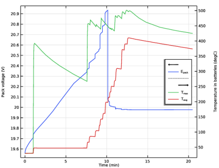
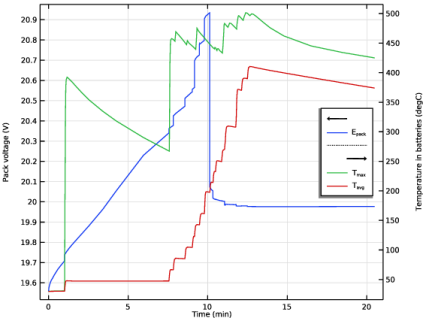
In the Settings window for 1D Plot Group, type Pack Voltage and Max Temperature Probes in the Label text field.
3
Locate the Plot Settings section. Select the Two y-axes check box.
4
In the table, select the Plot on secondary y-axis check box for Probe Table Graph 2.
5
Select the Secondary y-axis label check box. In the associated text field, type Temperature in batteries (degC).
6
Locate the Legend section. From the Position list, choose Middle right.
Probe Table Graph 1
1
In the Model Builder window, expand the Pack Voltage and Max Temperature Probes node, then click Probe Table Graph 1.
2
In the Settings window for Table Graph, click to expand the Legends section.
3
From the Legends list, choose Manual.
4
Probe Table Graph 2
1
In the Model Builder window, click Probe Table Graph 2.
2
In the Settings window for Table Graph, locate the Legends section.
3
From the Legends list, choose Manual.
4
5
In the Pack Voltage and Max Temperature Probes toolbar, click  Plot.
Animation 1
You may also create an animation of the temperature surface plot as follows:
1
In the Results toolbar, click  Animation and choose Player.
2
In the Settings window for Animation, locate the Scene section.
3
From the Subject list, choose Temperature (ht).
4
Locate the Animation Editing section. From the Time selection list, choose Interpolated.
5
In the Times (min) text field, type range(0,0.25,20).
6
Locate the Frames section. From the Frame selection list, choose All.
7
Click the  Play button in the Graphics toolbar.