PDF

Thermal Distribution in a Pack of Cylindrical Batteries
Introduction
This example demonstrates how to model the temperature distribution in a battery pack during a 4C discharge. The pack is constructed by first coupling two cylindrical batteries in parallel. Six parallel-connected pairs are then connected in series to create the full pack — a configuration also called 6s2p. This configuration for the lithium ion battery pack is quite common in portable devices like skateboards, toys, drones, and medical equipment. The symmetry of the problem is used twice so that only the temperature distribution for three batteries needs to be solved for.
A Battery Pack interface is used to generate the appropriate heat sources, which is then coupled to one Heat Transfer interface in a 3D geometry.
For a detailed description of the underlying battery model, see the Parameter Estimation of a Time-Dependent Lumped Battery Model tutorial.
Model Definition
Figure 1 shows the model geometry. Three 21,700 battery cylinders (21 mm in diameter, 70 mm high) are placed adjacent to each other. Small electrically conducting strips of aluminum are located at the top and bottom of the cylinders according to the 6s2p configuration. The whole pack is assumed to be wrapped in plastic, forming a domain filled with air. Assuming a nominal charge capacity of 4 Ah for each cell and nominal voltage of 3.7 V, the battery pack has a total nominal capacity of approximately 178 Wh.
Figure 1: Model geometry.
The Battery Pack interface is used to define separate (lumped) battery models for each battery cylinder, with temperature-dependent ohmic, exchange current and diffusion time-constant parameters according to Arrhenius expressions. The Battery Pack interface also models the electric potential in the electric conductors use to connect the batteries.
The temperature profile is modeled using a Heat Transfer interface, where the heat sources stemming from the battery models, and the joule heating in the electric conductors, are included by the use of an Electrochemical Heating multiphysics node. The convection in the air-filled domain enclosing the batteries is neglected, assuming quiescent conditions. The outer boundaries of the pack are cooled using a convective cooling condition. Symmetry (no flux) conditions are used for the interior flat symmetry boundaries facing the rest of the pack.
Anisotropic heat conductivities are used in each battery by the use of the Battery Layers node, which makes use of individual cylindrical coordinate systems for each battery cylinder, with generally lower heat conductivities in the through-layer (radial) direction compared to the in-layer (angular and z) directions - a result of the spirally wound metal foils in the jelly roll design of the batteries.
The pack is discharged from 100% to 20% state-of-charge (SOC) using a 4C rate for 12 minutes.
Results and Discussion
Figure 2 shows the temperature distribution in the pack at the end of the simulation, where the solution data has been mirrored twice to illustrate the temperature of the full 6s2p pack. The innermost parts of the pack experience a temperature about 2°C higher than the outermost parts.
Figure 2: Temperature plot at t= 0.2 h.
Figure 3 shows a plot of the individual cell voltages during the discharge. The outermost cell (Cell 1) exhibits a slightly lower discharge voltage, a result of the ohmic drop and exchange current being slightly lower, and the diffusion time constant slightly higher, for the lower temperature, but the effect is small. The corresponding temperatures are shown in Figure 4.
Figure 3: Cell voltages versus time.
Figure 4: Average cell temperatures versus time.
Application Library path: Battery_Design_Module/Thermal_Management/battery_pack_6s2p
Modeling Instructions
From the File menu, choose New.
New
In the New window, click  Model Wizard.
Model Wizard
1
In the Model Wizard window, Start with adding a 3D space dimension along with a Heat Transfer in Fluids and a Battery Pack interface.
2
3
In the Select Physics tree, select Electrochemistry>Batteries>Battery Pack (bp).
4
Click Add.
5
In the Select Physics tree, select Heat Transfer>Heat Transfer in Fluids (ht).
6
Click Add.
7
Click  Study.
8
In the Select Study tree, select General Studies>Time Dependent.
9
Definitions
Add an analytical function to account for the temperature dependent activation energy using the Arrhenius relation.
Analytic 1 (an1)
1
In the Home toolbar, click  Functions and choose Local>Analytic.
2
In the Settings window for Analytic, type Arrh in the Function name text field.
3
Locate the Definition section. In the Expression text field, type exp(Ea/R_const*(1/Temp-1/T0)).
4
In the Arguments text field, type Ea, Temp.
5
Locate the Units section. In the table, enter the following settings:
6
In the Function text field, type 1.
E_OCP
Next add interpolation functions to define the SOC dependent equilibrium potential and its temperature dependence.
1
In the Home toolbar, click  Functions and choose Local>Interpolation.
2
In the Settings window for Interpolation, type E_OCP in the Label text field.
3
Locate the Definition section. From the Data source list, choose File.
4
In the Filename text field, type battery_pack_6s2p_E_OCP_data.txt.
5
Locate the Units section. In the Argument table, enter the following settings:
6
In the Function table, enter the following settings:
dEdT
1
In the Home toolbar, click  Functions and choose Local>Interpolation.
2
In the Settings window for Interpolation, type dEdT in the Label text field.
3
Locate the Definition section. From the Data source list, choose File.
4
In the Filename text field, type battery_pack_6s2p_dEdT_data.txt.
5
Locate the Units section. In the Argument table, enter the following settings:
6
In the Function table, enter the following settings:
Geometry 1
The model geometry is available as a parameterized geometry sequence in a separate MPH-file. If you want to build it from scratch, follow the instructions in the section Appendix — Geometry Modeling Instructions. Otherwise load it from file with the following steps.
1
In the Geometry toolbar, click Insert Sequence and choose Insert Sequence.
2
3
In the Geometry toolbar, click  Build All.
4
Click the  Transparency button in the Graphics toolbar.
5
Click the  Zoom Extents button in the Graphics toolbar.
Global Definitions
Geometry Parameters
1
In the Model Builder window, under Global Definitions click Parameters 1.
2
In the Settings window for Parameters, type Geometry Parameters in the Label text field.
Battery Parameters
Add the parameter file required for setting up the physics of the lumped battery and heat transfer interfaces.
1
In the Home toolbar, click  Parameters and choose Add>Parameters.
2
In the Settings window for Parameters, type Battery Parameters in the Label text field.
3
Locate the Parameters section. Click  Load from File.
4
Materials
Next, add and define the materials in the different domains: air to the region surrounding the batteries and aluminum to the current collectors.
Add Material
1
In the Home toolbar, click  Add Material to open the Add Material window.
2
Go to the Add Material window.
3
4
Click Add to Component in the window toolbar.
5
In the tree, select Built-in>Aluminum.
6
Click Add to Component in the window toolbar.
7
In the Home toolbar, click  Add Material to close the Add Material window.
Materials
Air (mat1)
1
In the Model Builder window, under Component 1 (comp1)>Materials click Air (mat1).
2
In the Settings window for Material, locate the Geometric Entity Selection section.
3
From the Selection list, choose Air Domain.
Aluminum (mat2)
1
In the Model Builder window, click Aluminum (mat2).
2
In the Settings window for Material, locate the Geometric Entity Selection section.
3
From the Selection list, choose Conductors.
Battery Pack (bp)
Now define the batteries of the pack.
1
In the Model Builder window, under Component 1 (comp1) click Battery Pack (bp).
2
In the Settings window for Battery Pack, locate the Domain Selection section.
3
From the Selection list, choose Batteries and Conductors.
Batteries
1
In the Model Builder window, under Component 1 (comp1)>Battery Pack (bp) click Batteries.
2
In the Settings window for Batteries, locate the Domain Selection section.
3
From the Selection list, choose Batteries.
4
Locate the Battery Pack Settings section. In the Qpack,0 text field, type 3*Q_cell.
5
In the SOCpack,0 text field, type 1.
Cell Equilibrium Potential 1
1
In the Model Builder window, click Cell Equilibrium Potential 1.
2
In the Settings window for Cell Equilibrium Potential, locate the Open Circuit Voltage section.
3
From the Open circuit voltage input list, choose From definitions.
4
From the EOCV,ref list, choose E_OCP (int1).
5
From the dEOCV/dT list, choose dEdT (int2).
Voltage Losses 1
1
In the Model Builder window, click Voltage Losses 1.
2
In the Settings window for Voltage Losses, locate the Ohmic Overpotential section.
3
In the ηIR,1C text field, type eta_1C*Arrh(Ea_eta1C, bp.T_cell).
4
Locate the Activation Overpotential section. In the J0 text field, type J0_0*Arrh(Ea_J0,bp.T_cell).
5
Locate the Concentration Overpotential section. Select the Include concentration overpotential check box.
6
In the τ text field, type tau_0*Arrh(Ea_Tau,bp.T_cell).
Current Conductors
1
In the Model Builder window, under Component 1 (comp1)>Battery Pack (bp) click Current Conductors.
2
In the Settings window for Current Conductors, locate the Domain Selection section.
3
From the Selection list, choose Conductors.
Ground 1
1
In the Physics toolbar, click  Attributes and choose Ground.
2
Current Conductors
In the Model Builder window, click Current Conductors.
Current 1
1
In the Physics toolbar, click  Attributes and choose Current.
2
3
In the Settings window for Current, locate the Electrode Current section.
4
In the Is,total text field, type -I_1C*C_rate.
Negative Connectors
1
In the Model Builder window, under Component 1 (comp1)>Battery Pack (bp) click Negative Connectors.
2
Positive Connectors
1
In the Model Builder window, click Positive Connectors.
2
Heat Transfer in Fluids (ht)
Now define the heat transfer in the battery pack.
Initial Values 1
1
In the Model Builder window, under Component 1 (comp1)>Heat Transfer in Fluids (ht) click Initial Values 1.
2
In the Settings window for Initial Values, locate the Initial Values section.
3
In the T text field, type T_init.
Heat Flux 1
1
In the Physics toolbar, click  Boundaries and choose Heat Flux.
2
In the Settings window for Heat Flux, locate the Boundary Selection section.
3
From the Selection list, choose Heat Flux Boundaries.
4
Locate the Heat Flux section. From the Flux type list, choose Convective heat flux.
5
In the h text field, type ht.
6
In the Text text field, type T_init.
Battery Layers 1
1
In the Physics toolbar, click  Domains and choose Battery Layers.
2
In the Settings window for Battery Layers, locate the Domain Selection section.
3
From the Selection list, choose Batteries.
Due to the winding of the layers, the thermal conductivities in the battery domains exhibit anisotropic properties, with higher conductivity values in the in-layer direction compared to the through-layer (radial) direction.
4
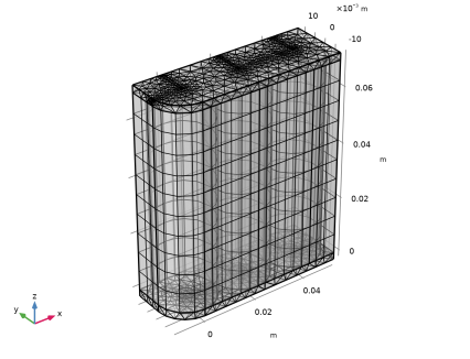
Locate the Battery Layers section. From the Layer configuration list, choose Spirally wound (cylindrical).
5
In the ktl text field, type kT_batt_tl.
6
In the kil text field, type kT_batt_il.
7
In the ρeff text field, type rho_batt.
8
In the Cp,eff text field, type Cp_batt.
Solid 1
1
In the Physics toolbar, click  Domains and choose Solid.
2
In the Settings window for Solid, locate the Domain Selection section.
3
From the Selection list, choose Conductors.
Multiphysics
Add a two-way coupling between the Battery Pack and the Heat Transfer interfaces for the heat sources and the temperature by adding an Electrochemical Heating multiphysics node.
Electrochemical Heating 1 (ech1)
In the Physics toolbar, click  Multiphysics Couplings and choose Domain>Electrochemical Heating.
Mesh 1
Swept 1
1
In the Mesh toolbar, click  Swept.
2
In the Settings window for Swept, locate the Domain Selection section.
3
From the Geometric entity level list, choose Domain.
4
From the Selection list, choose Mesh Sweep Domains.
5
Click to expand the Sweep Method section. From the Face meshing method list, choose Triangular (generate prisms).
Free Tetrahedral 1
1
In the Mesh toolbar, click  Free Tetrahedral.
2
In the Model Builder window, right-click Mesh 1 and choose Build All.
Definitions (comp1)
Adding probes for temperatures and cell potentials allows for visualizing results while solving. The Battery Pack interface defines cell potential variables named bp.E_cell_X and bp.T_cell_X for the individual cell voltages and volume-averaged cell temperatures, where X represents the cell number. Add probes for these variables as follows:
Temperature Cell 1
1
In the Definitions toolbar, click  Probes and choose Global Variable Probe.
2
In the Settings window for Global Variable Probe, type Temp1 in the Variable name text field.
3
In the Label text field, type Temperature Cell 1.
4
Locate the Expression section. In the Expression text field, type bp.T_cell_1.
5
From the Table and plot unit list, choose degC.
6
Select the Description check box. In the associated text field, type Cell 1.
7
Click to expand the Table and Window Settings section. Click  Add Table.
8
From the Plot window list, choose New window.
9
Click  Add Plot Window.
Temperature Cell 2
1
Right-click Temperature Cell 1 and choose Duplicate.
2
In the Settings window for Global Variable Probe, type Temperature Cell 2 in the Label text field.
3
In the Variable name text field, type Temp2.
4
Locate the Expression section. In the Expression text field, type bp.T_cell_2.
5
In the Description text field, type Cell 2.
Temperature Cell 3
1
Right-click Temperature Cell 2 and choose Duplicate.
2
In the Settings window for Global Variable Probe, type Temperature Cell 3 in the Label text field.
3
In the Variable name text field, type Temp3.
4
Locate the Expression section. In the Expression text field, type bp.T_cell_2.
5
In the Description text field, type Cell 3.
Cell Potential 1
1
Right-click Temperature Cell 3 and choose Duplicate.
2
In the Settings window for Global Variable Probe, type Cell Potential 1 in the Label text field.
3
In the Variable name text field, type Ecell1.
4
Locate the Expression section. In the Expression text field, type bp.E_cell_1.
5
In the Description text field, type Cell 1.
6
Locate the Table and Window Settings section. Click  Add Table.
7
From the Plot window list, choose New window.
8
Click  Add Plot Window.
Cell Potential 2
1
Right-click Cell Potential 1 and choose Duplicate.
2
In the Settings window for Global Variable Probe, type Cell Potential 2 in the Label text field.
3
In the Variable name text field, type Ecell2.
4
Locate the Expression section. In the Expression text field, type bp.E_cell_2.
5
In the Description text field, type Cell 2.
Cell Potential 3
1
Right-click Cell Potential 2 and choose Duplicate.
2
In the Settings window for Global Variable Probe, type Cell Potential 3 in the Label text field.
3
In the Variable name text field, type Ecell3.
4
Locate the Expression section. In the Expression text field, type bp.E_cell_3.
5
In the Description text field, type Cell 3.
Study 1
Step 1: Time Dependent
1
In the Model Builder window, under Study 1 click Step 1: Time Dependent.
2
In the Settings window for Time Dependent, locate the Study Settings section.
3
From the Time unit list, choose h.
4
In the Output times text field, type 0 0.8/C_rate.
5
In the Home toolbar, click  Compute.
Results
Add a dataset with a selection and mirror it twice in order to visualize the temperature of the full 6s2p configuration.
Study 1/Solution 1 (3) (sol1)
In the Results toolbar, click  More Datasets and choose Solution.
Selection
1
In the Results toolbar, click  Attributes and choose Selection.
2
In the Settings window for Selection, locate the Geometric Entity Selection section.
3
From the Geometric entity level list, choose Domain.
4
From the Selection list, choose Batteries and Conductors.
Mirror 3D 1
1
In the Results toolbar, click  More Datasets and choose Mirror 3D.
2
In the Settings window for Mirror 3D, locate the Data section.
3
From the Dataset list, choose Study 1/Solution 1 (3) (sol1).
4
Locate the Plane Data section. In the X-coordinate text field, type 2.5*(d_batt).
Mirror 3D 2
1
Right-click Mirror 3D 1 and choose Duplicate.
2
In the Settings window for Mirror 3D, locate the Data section.
3
From the Dataset list, choose Mirror 3D 1.
4
Locate the Plane Data section. From the Plane list, choose zx-planes.
5
In the y-coordinate text field, type d_batt/2.
6
Cell Temperatures vs. Time
1
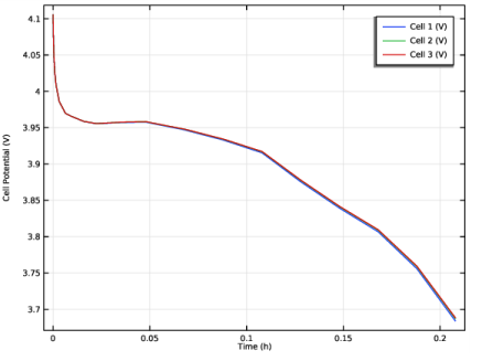
In the Model Builder window, expand the Results>Probe Plot Group 6 node, then click Probe Plot Group 6.
2
In the Settings window for 1D Plot Group, type Cell Temperatures vs. Time in the Label text field.
3
Locate the Plot Settings section. Select the x-axis label check box.
4
Select the y-axis label check box. In the associated text field, type Cell Temperature (degC).
5
Locate the Legend section. From the Position list, choose Lower right.
6
In the Cell Temperatures vs. Time toolbar, click  Plot.
Cell Potential vs. Time
1
In the Model Builder window, under Results click Probe Plot Group 7.
2
In the Settings window for 1D Plot Group, type Cell Potential vs. Time in the Label text field.
3
Locate the Plot Settings section. Select the x-axis label check box.
4
Select the y-axis label check box. In the associated text field, type Cell Potential (V).
5
In the Cell Potential vs. Time toolbar, click  Plot.
Temperature
1
In the Home toolbar, click  Add Plot Group and choose 3D Plot Group.
2
In the Settings window for 3D Plot Group, locate the Data section.
3
From the Dataset list, choose Mirror 3D 2.
4
In the Label text field, type Temperature.
Surface 1
1
Right-click Temperature and choose Surface.
2
In the Settings window for Surface, click Replace Expression in the upper-right corner of the Expression section. From the menu, choose Component 1 (comp1)>Heat Transfer in Fluids>Temperature>T - Temperature - K.
3
Locate the Expression section. From the Unit list, choose degC.
4
Locate the Coloring and Style section. Click  Change Color Table.
5
In the Color Table dialog box, select Thermal>HeatCameraLight in the tree.
6
7
In the Temperature toolbar, click  Plot.
8
Click the  Zoom Extents button in the Graphics toolbar.
 
Appendix — Geometry Modeling Instructions
From the File menu, choose New.
New
In the New window, click  Model Wizard.
Model Wizard
1
In the Model Wizard window, click  3D.
2
Global Definitions
Geometry Parameters
1
In the Model Builder window, under Global Definitions click Parameters 1.
2
In the Settings window for Parameters, type Geometry Parameters in the Label text field.
3
Locate the Parameters section. Click  Load from File.
4
Geometry 1
Cylinder 1 (cyl1)
1
In the Geometry toolbar, click  Cylinder.
2
In the Settings window for Cylinder, locate the Size and Shape section.
3
In the Radius text field, type r_batt.
4
In the Height text field, type h_batt.
Cylinder 2 (cyl2)
1
Right-click Cylinder 1 (cyl1) and choose Duplicate.
2
In the Settings window for Cylinder, locate the Size and Shape section.
3
In the Radius text field, type r_term.
4
In the Height text field, type h_term.
5
Locate the Position section. In the z text field, type -h_term.
Array 1 (arr1)
1
In the Geometry toolbar, click  Transforms and choose Array.
2
In the Settings window for Array, locate the Input section.
3
Click  Paste Selection.
4
In the Paste Selection dialog box, type cyl2 in the Selection text field.
5
6
In the Settings window for Array, click to collapse the Displacement section.
7
Locate the Size section. In the z size text field, type 2.
8
Click to expand the Displacement section. In the z text field, type h_batt+h_term.
Array 2 (arr2)
1
Right-click Array 1 (arr1) and choose Duplicate.
2
In the Settings window for Array, locate the Input section.
3
Find the Input objects subsection. Click to select the  Activate Selection toggle button.
4
Click  Paste Selection.
5
In the Paste Selection dialog box, type cyl1 in the Selection text field.
6
7
In the Settings window for Array, locate the Input section.
8
Click  Paste Selection.
9
In the Paste Selection dialog box, type arr1(1,1,1) in the Selection text field.
10
11
In the Settings window for Array, locate the Input section.
12
Click  Paste Selection.
13
In the Paste Selection dialog box, type arr1(1,1,2) in the Selection text field.
14
15
In the Settings window for Array, locate the Size section.
16
In the x size text field, type 3.
17
Locate the Displacement section. In the x text field, type d_batt.
18
In the z text field, type 0.
19
Click  Build Selected.
Block 1 (blk1)
1
In the Geometry toolbar, click  Block.
2
In the Settings window for Block, locate the Size and Shape section.
3
In the Width text field, type d_batt+d_sc.
4
In the Depth text field, type d_sc.
5
In the Height text field, type h_sc.
6
Locate the Position section. In the x text field, type -d_sc/2.
7
In the y text field, type -d_sc/2.
8
In the z text field, type -h_sc-h_term.
9
Click  Build Selected.
Block 2 (blk2)
1
In the Geometry toolbar, click  Block.
2
In the Settings window for Block, locate the Size and Shape section.
3
In the Width text field, type (d_batt+d_sc)/2.
4
In the Depth text field, type d_sc.
5
In the Height text field, type h_sc.
6
Locate the Position section. In the x text field, type -d_sc/2+(d_batt)*2.
7
In the y text field, type -d_sc/2.
8
In the z text field, type -h_term-h_sc.
Block 3 (blk3)
1
Right-click Block 2 (blk2) and choose Duplicate.
2
In the Settings window for Block, locate the Size and Shape section.
3
In the Width text field, type (d_batt)/2+d_sc.
4
Locate the Position section. In the x text field, type -d_sc/2-d_batt/2.
5
In the z text field, type h_batt+h_term.
Block 4 (blk4)
1
Right-click Block 3 (blk3) and choose Duplicate.
2
In the Settings window for Block, locate the Size and Shape section.
3
In the Width text field, type w_pc.
4
In the Depth text field, type d_batt/2+w_pc/2.
5
In the Height text field, type h_pc.
6
Locate the Position section. In the x text field, type -w_pc/2.
7
In the y text field, type -w_pc/2.
8
In the z text field, type -h_term-h_sc-h_pc.
9
Click  Build Selected.
Move 1 (mov1)
1
In the Geometry toolbar, click  Transforms and choose Move.
2
Click the  Zoom Extents button in the Graphics toolbar.
3
Click the  Transparency button in the Graphics toolbar.
4
In the Settings window for Move, locate the Input section.
5
Click  Paste Selection.
6
In the Paste Selection dialog box, type blk1 in the Selection text field.
7
8
In the Settings window for Move, locate the Input section.
9
Select the Keep input objects check box.
10
Locate the Displacement section. In the x text field, type d_batt.
11
In the z text field, type h_batt+h_term*2+h_sc.
12
Click the  Zoom Extents button in the Graphics toolbar.
Array 3 (arr3)
1
In the Geometry toolbar, click  Transforms and choose Array.
2
In the Settings window for Array, locate the Input section.
3
Click  Paste Selection.
4
In the Paste Selection dialog box, type blk4 in the Selection text field.
5
6
In the Settings window for Array, locate the Size section.
7
In the x size text field, type 3.
8
In the z size text field, type 2.
9
Locate the Displacement section. In the x text field, type d_batt.
10
In the z text field, type h_batt+2*(h_term+h_sc)+h_pc.
11
Click  Build Selected.
Move 1 (mov1)
1
In the Model Builder window, click Move 1 (mov1).
2
In the Settings window for Move, click  Build Selected.
3
Click  Build All Objects.
Work Plane 1 (wp1)
1
In the Geometry toolbar, click  Work Plane.
2
In the Settings window for Work Plane, locate the Plane Definition section.
3
In the z-coordinate text field, type -(h_term+h_sc+h_pc).
Work Plane 1 (wp1)>Plane Geometry
In the Model Builder window, click Plane Geometry.
Work Plane 1 (wp1)>Circle 1 (c1)
1
In the Work Plane toolbar, click  Circle.
2
In the Settings window for Circle, locate the Size and Shape section.
3
In the Radius text field, type r_batt.
4
In the Sector angle text field, type 90.
5
Locate the Rotation Angle section. In the Rotation text field, type 180.
Work Plane 1 (wp1)>Square 1 (sq1)
1
In the Work Plane toolbar, click  Square.
2
In the Settings window for Square, locate the Size section.
3
In the Side length text field, type r_batt.
4
Locate the Position section. In the xw text field, type -r_batt.
5
In the yw text field, type -r_batt.
Work Plane 1 (wp1)>Difference 1 (dif1)
1
In the Work Plane toolbar, click  Booleans and Partitions and choose Difference.
2
Click the  Zoom Extents button in the Graphics toolbar.
3
4
In the Settings window for Difference, locate the Difference section.
5
Find the Objects to subtract subsection. Click to select the  Activate Selection toggle button.
6
Click  Paste Selection.
7
In the Paste Selection dialog box, type c1 in the Selection text field.
8
9
In the Settings window for Difference, click  Build Selected.
Work Plane 1 (wp1)>Rectangle 1 (r1)
1
In the Work Plane toolbar, click  Rectangle.
2
In the Settings window for Rectangle, locate the Size and Shape section.
3
In the Width text field, type 3*(d_batt).
4
In the Height text field, type d_batt.
5
Click  Build Selected.
6
Locate the Position section. In the xw text field, type -r_batt.
7
In the yw text field, type -r_batt.
Work Plane 1 (wp1)>Difference 2 (dif2)
1
In the Work Plane toolbar, click  Booleans and Partitions and choose Difference.
2
3
In the Settings window for Difference, locate the Difference section.
4
Find the Objects to subtract subsection. Click to select the  Activate Selection toggle button.
5
Click the  Zoom Extents button in the Graphics toolbar.
6
7
Click  Build Selected.
Extrude 1 (ext1)
1
In the Model Builder window, right-click Geometry 1 and choose Extrude.
2
In the Settings window for Extrude, locate the Distances section.
3
4
Click  Build Selected.
Form Union (fin)
In the Geometry toolbar, click  Build All.
Battery 1
1
In the Geometry toolbar, click  Selections and choose Explicit Selection.
2
On the object fin, select Domain 4 only.
3
In the Settings window for Explicit Selection, type Battery 1 in the Label text field.
Battery 2
1
In the Geometry toolbar, click  Selections and choose Explicit Selection.
2
On the object fin, select Domain 14 only.
3
In the Settings window for Explicit Selection, type Battery 2 in the Label text field.
Battery 3
1
In the Geometry toolbar, click  Selections and choose Explicit Selection.
2
On the object fin, select Domain 22 only.
3
In the Settings window for Explicit Selection, type Battery 3 in the Label text field.
Air Domain
1
In the Geometry toolbar, click  Selections and choose Explicit Selection.
2
On the object fin, select Domains 2, 3, 5, 12, 13, 20, 21, 28, and 29 only.
3
In the Settings window for Explicit Selection, type Air Domain in the Label text field.
Conductors
1
In the Geometry toolbar, click  Selections and choose Complement Selection.
2
In the Settings window for Complement Selection, locate the Input Entities section.
3
4
In the Add dialog box, in the Selections to invert list, choose Battery 1, Battery 2, Battery 3, and Air Domain.
5
6
In the Settings window for Complement Selection, type Conductors in the Label text field.
7
In the Geometry toolbar, click  Build All.
Batteries
1
In the Geometry toolbar, click  Selections and choose Union Selection.
2
In the Settings window for Union Selection, locate the Input Entities section.
3
4
In the Add dialog box, in the Selections to add list, choose Battery 1, Battery 2, and Battery 3.
5
6
In the Settings window for Union Selection, type Batteries in the Label text field.
Batteries and Conductors
1
In the Geometry toolbar, click  Selections and choose Union Selection.
2
In the Settings window for Union Selection, locate the Input Entities section.
3
4
In the Add dialog box, in the Selections to add list, choose Conductors and Batteries.
5
6
In the Settings window for Union Selection, type Batteries and Conductors in the Label text field.
Heat Flux Boundaries
1
In the Geometry toolbar, click  Selections and choose Explicit Selection.
2
In the Settings window for Explicit Selection, locate the Entities to Select section.
3
From the Geometric entity level list, choose Boundary.
4
In the Label text field, type Heat Flux Boundaries.
5
Locate the Entities to Select section. Click  Paste Selection.
6
In the Paste Selection dialog box, type fin: 2-10, 14, 15, 22, 44, 49, 54, 56, 58, 92, 97, 103, 138, 143, 148 in the Selection text field.
7
8
Click the  Wireframe Rendering button in the Graphics toolbar.
9
Click the  Zoom Extents button in the Graphics toolbar.
10
In the Geometry toolbar, click  Build All.
Mesh Sweep Domains
1
In the Geometry toolbar, click  Selections and choose Box Selection.
2
In the Settings window for Box Selection, type Mesh Sweep Domains in the Label text field.
3
Locate the Box Limits section. In the z minimum text field, type -h_pc/2.
4
In the z maximum text field, type h_batt+h_pc/2.
5
Locate the Output Entities section. From the Include entity if list, choose Entity inside box.