PDF

Diffuse Double Layer
Introduction
Close to an electrode surface, ions in the electrolyte are attracted and repelled by unscreened excess charge on the electrode. This region is called the diffuse double layer. Its size is normally a few nanometers away from the electrode surface. The electrical interactions here mean that charge separation can occur, and the assumption of local electroneutrality is not valid. The study of the diffuse double layer is important to applications that consider very thin layers of electrolyte, such as electrochemical capacitors, atmospheric corrosion problems, ion-selective field effect transistors (ISFETs), and nanoelectrochemistry.
This example shows how to define a double layer model by combining the Transport of Diluted Species and Electrostatics physics interfaces to account for mass transfer and charge transfer, respectively. The model contains one charged electrode adjacent to bulk solution.
One of the simplest physical models of the double layer is the Gouy–Chapman–Stern (GCS) model. In Gouy–Chapman theory (Ref. 1, Ref. 2), the diffuse double layer is treated as a multiphysics coupling of the Nernst–Planck equations for mass transport of all of the ions, with Poisson’s equation (Gauss’s law) for the charge density and electric field. The combination of these equations is frequently referred to as the Poisson–Nernst–Planck (PNP) equations or Nernst–Planck–Poisson (NPP) equations.
Gouy–Chapman theory predicts the spatial extent of the diffuse double layer to be of the same order as the Debye length for the solution, defined for a monovalent binary electrolyte with concentration cbulk and solvent relative permittivity εr:
(1)
The Stern modification (Ref. 3) to the Gouy–Chapman theory additionally considers the electric field inside a plane called the outer Helmholtz plane (OHP). This is the plane of closest approach to the electrode for dissolved ions in solution, due to the finite size of the ions and surrounding solvent molecules. In the distance of a fraction of a nanometer between this plane and the electrode surface, Stern’s theory describes the electrolyte as a dielectric of constant permittivity. This uncharged region of the double layer is sometimes called the compact double layer.
When there is a low applied potential (< RT/F ~ 25 mV), the Gouy–Chapman–Stern theory has an analytical solution. The capacitance is predicted to be the same as for a parallel plate capacitor whose electrode separation is equal to the sum of the Stern layer size and the Debye length:
(2)
Model Definition
The model geometry is in 1D (a single interval between 0 and L) and consists of a single domain, representing the electrolyte phase from the electrode through the diffuse double layer, as far as the electroneutral bulk solution. The compact component of the double layer is handled using a boundary condition set at x = 0.
Domain equations
The concentrations, ci (SI unit: mol/m3, i=+,-), of two ions of opposite charge (+1/-1) are solved for in the electrolyte phase. The fluxes (Ji, SI unit: mol/(m2·s)) of the ions are described by the Nernst–Planck equation
with Di (SI unit: m2/s) being the diffusion coefficient, um,i (SI unit: s·mol/kg) the mobility, F (SI unit: C/mol) the Faraday constant, and (SI unit: V) the electric potential in the electrolyte phase.
Assume that there are no homogeneous reactions of the ions in the solution. Then, conservation of mass requires that, for both species:
For the potential, the Poisson equation (Gauss’s law) states
where ε is the permittivity (SI unit: F/m) and ρ the charge density (SI unit: C/m3). The charge density depends on the ion concentrations according to:
Boundary conditions
We choose the bulk solution as the ground condition for the electrolyte potential:
which is set at the outer boundary.
The ion concentrations are set to their bulk values at the outer boundary. Because bulk solution is electroneutral, the positive and negative ions have equal concentrations here.
From Gauss’s law, the electric field inside the compact double layer is constant because this layer is uncharged and has a uniform permittivity. Hence, according to the Stern theory for a compact double layer of a constant thickness, λS (SI unit: m), the following Robin-type boundary condition applies for the electrolyte potential:
where (SI unit: V) is the applied potential of the electrode, as measured against bulk solution, and n is the boundary normal vector, pointing outwards from the electrolyte domain.
For the case of a nonzero Stern layer thickness, the condition can be reformulated as a surface charge condition that depends on the potential difference, (SI unit: V), between the electrode potential and the electrolyte potential at the outer Helmholtz plane (x = 0):
where
The Surface Charge Density condition in Electrostatics is used to define the above condition. The problem is solved for a sweep of values of from 1 mV to 10 mV.
If the electrode is inert to electrolysis of the ions at the electrolyte-electrode interface, no flux of the ions into the electrode surface can occur. Hence, No Flux conditions are used for both ion concentrations at the electrode boundary.
Results and Discussion
Figure 1 shows the potential profile in the electrolyte as a line graph and the potential at the electrode as a point.
Figure 1: Electrolyte potential profile (blue line) and 10 mV applied electrode potential vs bulk solution (red dot).
The potential difference between the red dot (electrode surface) and the value of the blue line at x = 0 represents the potential difference over the compact double layer. The electrolyte potential falls off exponentially on the Debye length scale (Equation 1), as predicted by Gouy–Chapman theory.
Figure 2 shows the concentrations of the two ionic species. Because the electrode is polarized positively against bulk solution, it is positively charged and attracts anions while repelling cations. The concentration profiles confirm that the anion in the electrolyte is accumulated at the surface, while the cation is depleted.
Figure 2: Concentration profile for the two ions, showing cation depletion (blue line) and anion accumulation (green line).
Figure 3 shows the surface charge dependence on the applied potential. This agrees precisely with the low potential analytical expression (Equation 2) for the smaller potentials. At 10 mV applied potential, a small deviation is observed as the low potential approximation becomes less precise.
Figure 3: Surface charge density as a function of applied potential difference between the electrode and bulk solution, comparing simulation results with analytical theory derived in the limit of low applied potential.
References
1. L.G. Gouy, Comptes Rendues Hebdomadaires des Séances de l’Académie des Sciences, vol. 149, pp. 654–657, 1909.
2. D.L. Chapman, Philosophical Magazine, vol. 25, pp. 475–481, 1913.
3. O. Stern, Zeitschrift für Elektrochemie, vol. 30, pp. 508–516, 1924.
4. A.J. Bard and L.R. Faulkner, Electrochemical Methods: Fundamentals and Applications, 2nd ed., Hoboken, 2001.
Application Library path: Battery_Design_Module/General_Electrochemistry/diffuse_double_layer
Modeling Instructions
From the File menu, choose New.
New
In the New window, click  Model Wizard.
Model Wizard
1
In the Model Wizard window, click  1D.
2
In the Select Physics tree, select Chemical Species Transport>Nernst-Planck-Poisson Equations.
3
Click Add.
4
In the Electric potential text field, type phi.
5
In the Added physics interfaces tree, select Transport of Diluted Species (tds).
6
In the Number of species text field, type 2.
7
In the Concentrations table, enter the following settings:
8
Click  Study.
9
In the Select Study tree, select General Studies>Stationary.
10
Global Definitions
Start by loading some parameters from a text file.
Parameters 1
1
In the Model Builder window, under Global Definitions click Parameters 1.
2
In the Settings window for Parameters, locate the Parameters section.
3
Click  Load from File.
4
Definitions
Proceed by adding some variable expressions from a text file.
Variables 1
1
In the Model Builder window, under Component 1 (comp1) right-click Definitions and choose Variables.
2
In the Settings window for Variables, locate the Variables section.
3
Click  Load from File.
4
Geometry 1
Build the geometry as a single interval.
Interval 1 (i1)
1
In the Model Builder window, under Component 1 (comp1) right-click Geometry 1 and choose Interval.
2
In the Settings window for Interval, locate the Interval section.
3
4
Click  Build All Objects.
Electrostatics (es)
Now, add the required physics for this model. Begin with the Electrostatics physics (Poisson’s equation).
Charge Conservation 1
1
In the Model Builder window, under Component 1 (comp1)>Electrostatics (es) click Charge Conservation 1.
2
In the Settings window for Charge Conservation, locate the Constitutive Relation D-E section.
3
From the εr list, choose User defined. In the associated text field, type eps_H2O.
Surface Charge Density 1
1
In the Physics toolbar, click  Boundaries and choose Surface Charge Density.
2
3
In the Settings window for Surface Charge Density, locate the Surface Charge Density section.
4
In the ρs text field, type rho_surf.
Ground 1
1
In the Physics toolbar, click  Boundaries and choose Ground.
2
Transport of Diluted Species (tds)
Now set up the model for the transport of the ions.
Species Charges
1
In the Model Builder window, under Component 1 (comp1)>Transport of Diluted Species (tds) click Species Charges.
2
In the Settings window for Species Properties, locate the Charge section.
3
In the zcA text field, type zA.
4
In the zcX text field, type zX.
Transport Properties 1
1
In the Model Builder window, click Transport Properties 1.
2
In the Settings window for Transport Properties, locate the Diffusion section.
3
In the DcA text field, type DA.
4
In the DcX text field, type DX.
Initial Values 1
1
In the Model Builder window, click Initial Values 1.
2
In the Settings window for Initial Values, locate the Initial Values section.
3
In the cA text field, type cA_bulk.
4
In the cX text field, type cX_bulk.
Concentration 1
1
In the Physics toolbar, click  Boundaries and choose Concentration.
2
3
In the Settings window for Concentration, locate the Concentration section.
4
Select the Species cA check box.
5
In the c0,cA text field, type cA_bulk.
6
Select the Species cX check box.
7
In the c0,cX text field, type cX_bulk.
Define the temperature in the system.
Global Definitions
Default Model Inputs
1
In the Model Builder window, under Global Definitions click Default Model Inputs.
2
In the Settings window for Default Model Inputs, locate the Browse Model Inputs section.
3
In the tree, select General>Temperature (K) - minput.T.
4
Find the Expression for remaining selection subsection. In the Temperature text field, type T0.
Mesh 1
Edit the default meshing sequence. The mesh parameters are dependent of the Debye length to make sure that the mesh is always well resolved.
1
In the Model Builder window, under Component 1 (comp1) click Mesh 1.
2
In the Settings window for Mesh, locate the Sequence Type section.
3
From the list, choose User-controlled mesh.
Size 1
1
In the Model Builder window, right-click Edge 1 and choose Size.
2
In the Settings window for Size, locate the Element Size section.
3
Click the Custom button.
4
Locate the Element Size Parameters section.
5
Select the Maximum element size check box. In the associated text field, type h_max.
Size 2
1
Right-click Edge 1 and choose Size.
2
In the Settings window for Size, locate the Geometric Entity Selection section.
3
From the Geometric entity level list, choose Boundary.
4
5
Locate the Element Size section. Click the Custom button.
6
Locate the Element Size Parameters section.
7
Select the Maximum element size check box. In the associated text field, type h_max_surf.
8
Click  Build All.
Solve the problem using Auxiliary sweep for a range of potentials.
Study 1
Step 1: Stationary
1
In the Model Builder window, under Study 1 click Step 1: Stationary.
2
In the Settings window for Stationary, click to expand the Study Extensions section.
3
Select the Auxiliary sweep check box.
4
5
6
In the Home toolbar, click  Compute.
Results
Electric Potential (es)
Reproduce the figures from the Results and Discussion section as follows:
1
In the Settings window for 1D Plot Group, locate the Data section.
2
From the Parameter selection (phiM) list, choose Last.
3
Locate the Plot Settings section. Select the y-axis label check box.
Line Graph 1
1
In the Model Builder window, expand the Electric Potential (es) node, then click Line Graph 1.
2
In the Settings window for Line Graph, locate the x-Axis Data section.
3
From the Parameter list, choose Expression.
4
In the Expression text field, type x/xD.
5
Select the Description check box. In the associated text field, type Length (unit Debye lengths).
6
Click to expand the Legends section. Select the Show legends check box.
7
From the Legends list, choose Manual.
8
Point Graph 1
1
In the Model Builder window, right-click Electric Potential (es) and choose Point Graph.
2
Click the  Zoom Extents button in the Graphics toolbar.
3
4
In the Settings window for Point Graph, locate the y-Axis Data section.
5
In the Expression text field, type phiM.
6
Locate the x-Axis Data section. From the Parameter list, choose Expression.
7
In the Expression text field, type x/xD.
8
Select the Description check box. In the associated text field, type Length (unit Debye lengths).
9
Click to expand the Coloring and Style section. Find the Line style subsection. From the Line list, choose None.
10
From the Color list, choose Red.
11
Find the Line markers subsection. From the Marker list, choose Point.
12
Click to expand the Legends section. Select the Show legends check box.
13
From the Legends list, choose Manual.
14
15
In the Electric Potential (es) toolbar, click  Plot.
Concentrations, All Species (tds)
1
In the Model Builder window, under Results click Concentrations, All Species (tds).
2
In the Settings window for 1D Plot Group, locate the Data section.
3
From the Parameter selection (phiM) list, choose Last.
4
Click to expand the Title section. From the Title type list, choose None.
Species A
1
In the Model Builder window, expand the Concentrations, All Species (tds) node, then click Species A.
2
In the Settings window for Line Graph, locate the x-Axis Data section.
3
From the Unit list, choose nm.
4
Click to expand the Legends section. From the Legends list, choose Manual.
5
Species X
1
In the Model Builder window, click Species X.
2
In the Settings window for Line Graph, locate the x-Axis Data section.
3
From the Unit list, choose nm.
4
Locate the Legends section. From the Legends list, choose Manual.
5
6
In the Concentrations, All Species (tds) toolbar, click  Plot.
Line Graph 1
1
In the Model Builder window, expand the Results>Concentration, A (tds) node, then click Line Graph 1.
2
In the Settings window for Line Graph, click to expand the Coloring and Style section.
3
Find the Line markers subsection. From the Marker list, choose Cycle.
4
In the Number text field, type 1.
5
Click to expand the Legends section. Select the Show legends check box.
To more easily distinguish the lines from each other, Color Expression is used.
Color Expression 1
1
Right-click Line Graph 1 and choose Color Expression.
2
In the Settings window for Color Expression, locate the Expression section.
3
In the Expression text field, type phiM.
4
In the Concentration, A (tds) toolbar, click  Plot.
Concentration, A (tds)
1
In the Model Builder window, under Results click Concentration, A (tds).
2
In the Settings window for 1D Plot Group, locate the Legend section.
3
From the Layout list, choose Outside graph axis area.
Line Graph 1
1
In the Model Builder window, expand the Results>Concentration, X (tds) node, then click Line Graph 1.
2
In the Settings window for Line Graph, click to expand the Legends section.
3
Select the Show legends check box.
4
Locate the Coloring and Style section. Find the Line markers subsection. From the Marker list, choose Cycle.
5
In the Number text field, type 1.
Color Expression 1
1
Right-click Line Graph 1 and choose Color Expression.
2
In the Settings window for Color Expression, locate the Expression section.
3
In the Expression text field, type phiM.
4
In the Concentration, X (tds) toolbar, click  Plot.
Concentration, X (tds)
1
In the Model Builder window, under Results click Concentration, X (tds).
2
In the Settings window for 1D Plot Group, locate the Legend section.
3
From the Layout list, choose Outside graph axis area.
Surface Charge Density
1
In the Home toolbar, click  Add Plot Group and choose 1D Plot Group.
2
In the Settings window for 1D Plot Group, type Surface Charge Density in the Label text field.
3
Locate the Title section. From the Title type list, choose None.
Point Graph 1
1
Right-click Surface Charge Density and choose Point Graph.
2
3
In the Settings window for Point Graph, locate the y-Axis Data section.
4
In the Expression text field, type rho_surf.
5
Locate the x-Axis Data section. From the Parameter list, choose Expression.
6
In the Expression text field, type phiM.
7
Locate the Coloring and Style section. Find the Line style subsection. From the Line list, choose None.
8
Find the Line markers subsection. From the Marker list, choose Circle.
9
Click to expand the Legends section. Select the Show legends check box.
10
From the Legends list, choose Manual.
11
12
In the Surface Charge Density toolbar, click  Plot.
Global 1
1
In the Model Builder window, right-click Surface Charge Density and choose Global.
2
In the Settings window for Global, locate the y-Axis Data section.
3
4
Locate the x-Axis Data section. From the Parameter list, choose Expression.
5
In the Expression text field, type phiM.
Surface Charge Density
1
In the Model Builder window, click Surface Charge Density.
2
In the Settings window for 1D Plot Group, locate the Plot Settings section.
3
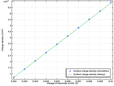
Select the y-axis label check box. In the associated text field, type Charge density (C/m<sup>2</sup>).
4
Locate the Legend section. From the Position list, choose Lower right.
5
In the Surface Charge Density toolbar, click  Plot.