|
|
|
|
1
|
|
2
|
In the Select Physics tree, select Acoustics>Pressure Acoustics>Pressure Acoustics, Frequency Domain (acpr).
|
|
3
|
Click Add.
|
|
4
|
In the Select Physics tree, select Acoustics>Pressure Acoustics>Pressure Acoustics, Boundary Elements (pabe).
|
|
5
|
Click Add.
|
|
6
|
|
7
|
Click Add.
|
|
8
|
|
9
|
Click Add.
|
|
10
|
Click
|
|
11
|
|
12
|
Click
|
|
1
|
|
2
|
|
3
|
|
1
|
|
2
|
|
3
|
Click
|
|
4
|
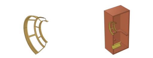
Browse to the model’s Application Libraries folder and double-click the file vented_loudspeaker_enclosure.mphbin.
|
|
5
|
Click
|
|
1
|
|
2
|
Select the object imp1 only.
|
|
3
|
|
4
|
|
5
|
|
1
|
|
2
|
|
3
|
|
4
|
|
5
|
|
1
|
|
2
|
|
3
|
|
4
|
|
5
|
|
6
|
|
7
|
|
8
|
|
9
|
|
10
|
|
11
|
Click
|
|
1
|
|
2
|
|
3
|
|
1
|
|
2
|
|
3
|
|
1
|
|
2
|
|
1
|
|
2
|
|
1
|
|
2
|
|
1
|
|
2
|
|
1
|
|
2
|
|
1
|
|
2
|
|
3
|
|
4
|
|
5
|
Click OK.
|
|
6
|
|
7
|
|
8
|
In the Add dialog box, in the Selections to subtract list, choose Coil, Soft Iron, Ferrite, and Enclosure.
|
|
9
|
Click OK.
|
|
1
|
|
2
|
|
3
|
|
4
|
In the Add dialog box, in the Selections to add list, choose Coil, Soft Iron, Ferrite, and Enclosure.
|
|
5
|
Click OK.
|
|
1
|
|
2
|
|
3
|
|
4
|
In the Add dialog box, in the Selections to add list, choose Coil, Narrow Region Inner, Narrow Region Outer, and Enclosure.
|
|
5
|
Click OK.
|
|
1
|
|
2
|
|
3
|
|
4
|
|
1
|
|
2
|
|
3
|
|
1
|
|
2
|
|
3
|
|
1
|
|
2
|
|
3
|
|
1
|
|
2
|
|
3
|
|
1
|
|
2
|
|
3
|
|
1
|
|
2
|
|
3
|
|
1
|
|
2
|
|
3
|
|
1
|
|
2
|
|
3
|
|
4
|
|
5
|
In the Add dialog box, in the Selections to add list, choose Composite, Cloth, Foam, Glass Fiber, and Basket.
|
|
6
|
Click OK.
|
|
1
|
|
2
|
|
3
|
|
4
|
|
5
|
|
1
|
|
2
|
In the Settings window for Difference, type Boundaries out of Symmetry Plane in the Label text field.
|
|
3
|
|
4
|
|
5
|
|
6
|
Click OK.
|
|
7
|
|
8
|
|
9
|
|
10
|
Click OK.
|
|
1
|
|
2
|
|
3
|
|
4
|
|
5
|
In the Add dialog box, in the Selections to add list, choose Cloth, Foam, Glass Fiber, and Other Mapped Boundaries.
|
|
6
|
Click OK.
|
|
7
|
|
8
|
|
9
|
|
10
|
Click OK.
|
|
1
|
|
2
|
|
3
|
|
4
|
|
5
|
|
1
|
|
2
|
|
3
|
|
4
|
Click
|
|
5
|
Browse to the model’s Application Libraries folder and double-click the file vented_loudspeaker_enclosure_Rb.txt.
|
|
6
|
Click
|
|
7
|
|
8
|
|
9
|
In the Function table, enter the following settings:
|
|
1
|
|
2
|
|
3
|
|
4
|
Click
|
|
5
|
Browse to the model’s Application Libraries folder and double-click the file vented_loudspeaker_enclosure_Lb.txt.
|
|
6
|
Click
|
|
7
|
|
8
|
|
9
|
In the Function table, enter the following settings:
|
|
1
|
|
2
|
|
3
|
|
1
|
|
2
|
|
1
|
|
2
|
|
1
|
|
2
|
|
3
|
In the tree, select Built-in>Air.
|
|
4
|
|
5
|
|
6
|
|
7
|
|
8
|
|
1
|
In the Material Browser window, In the ribbon make sure to select the Materials tab and then click the Browse Materials icon.
|
|
2
|
|
3
|
Browse to the model’s Application Libraries folder and double-click the file loudspeaker_driver_materials.mph.
|
|
4
|
Click
|
|
1
|
|
2
|
|
3
|
|
4
|
|
5
|
|
6
|
|
7
|
|
8
|
|
9
|
|
10
|
|
11
|
|
12
|
|
13
|
|
14
|
|
15
|
|
16
|
|
1
|
|
2
|
|
3
|
|
1
|
|
2
|
|
3
|
|
1
|
|
2
|
|
3
|
|
4
|
|
1
|
|
2
|
|
3
|
|
4
|
|
1
|
|
2
|
|
3
|
|
4
|
|
1
|
|
2
|
|
3
|
|
4
|
|
1
|
|
2
|
|
3
|
|
1
|
|
2
|
|
3
|
|
4
|
|
1
|
|
2
|
|
3
|
|
1
|
|
2
|
|
3
|
|
1
|
In the Model Builder window, under Component 1 (comp1) click Pressure Acoustics, Frequency Domain (acpr).
|
|
2
|
In the Settings window for Pressure Acoustics, Frequency Domain, locate the Domain Selection section.
|
|
3
|
|
1
|
|
2
|
|
3
|
|
1
|
|
2
|
|
3
|
|
4
|
|
5
|
|
1
|
|
2
|
|
3
|
|
4
|
|
5
|
|
1
|
In the Model Builder window, under Component 1 (comp1) click Pressure Acoustics, Boundary Elements (pabe).
|
|
2
|
In the Settings window for Pressure Acoustics, Boundary Elements, locate the Domain Selection section.
|
|
3
|
|
4
|
Click to expand the Symmetry/Infinite Boundary Condition section. From the Condition for the y = y0 plane list, choose Symmetric/Infinite sound hard boundary.
|
|
1
|
|
2
|
|
3
|
|
1
|
|
2
|
|
3
|
|
1
|
|
2
|
|
3
|
|
1
|
|
2
|
|
3
|
|
4
|
|
5
|
|
1
|
|
2
|
|
3
|
|
4
|
|
5
|
|
1
|
|
2
|
|
3
|
|
1
|
|
2
|
|
3
|
|
4
|
|
1
|
|
2
|
|
3
|
|
4
|
|
1
|
|
2
|
|
3
|
|
4
|
|
1
|
|
2
|
|
3
|
|
1
|
|
2
|
|
3
|
|
4
|
|
1
|
|
2
|
|
3
|
|
4
|
|
1
|
|
2
|
|
3
|
|
4
|
|
1
|
|
2
|
|
3
|
|
4
|
|
1
|
|
2
|
|
3
|
|
1
|
|
2
|
|
1
|
|
2
|
|
1
|
In the Physics toolbar, click
|
|
2
|
|
3
|
|
1
|
In the Physics toolbar, click
|
|
2
|
|
3
|
|
4
|
|
1
|
In the Physics toolbar, click
|
|
2
|
|
3
|
|
4
|
Locate the Coupled Interfaces section. From the Acoustics list, choose Pressure Acoustics, Boundary Elements (pabe).
|
|
1
|
In the Physics toolbar, click
|
|
2
|
|
3
|
|
4
|
Locate the Coupled Interfaces section. From the Acoustics list, choose Pressure Acoustics, Boundary Elements (pabe).
|
|
5
|
|
1
|
|
1
|
In the Physics toolbar, click
|
|
2
|
|
3
|
|
1
|
|
2
|
|
3
|
|
1
|
|
3
|
|
4
|
|
1
|
|
3
|
|
4
|
|
1
|
|
3
|
|
4
|
|
1
|
|
3
|
|
4
|
|
1
|
|
2
|
|
3
|
Click the Custom button.
|
|
4
|
|
5
|
|
1
|
|
2
|
|
3
|
|
4
|
|
1
|
|
3
|
|
4
|
|
1
|
|
2
|
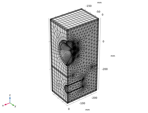
In the Settings window for Free Tetrahedral, click to expand the Element Quality Optimization section.
|
|
3
|
|
1
|
|
2
|
|
3
|
|
4
|
|
5
|
|
6
|
|
7
|
|
8
|
|
1
|
|
2
|
|
3
|
|
1
|
|
2
|
|
3
|
Click
|
|
4
|
|
5
|
|
6
|
|
7
|
|
8
|
Click Replace.
|
|
9
|
|
10
|
|
11
|
Right-click Study 1 - Complete Study>Step 1: Frequency Domain and choose Get Initial Value for Step.
|
|
1
|
In the Model Builder window, expand the Study 1 - Complete Study>Solver Configurations>Solution 1 (sol1)>Stationary Solver 1 node.
|
|
2
|
|
3
|
|
1
|
|
2
|
|
3
|
|
4
|
|
5
|
|
6
|
|
7
|
|
8
|
|
9
|
|
10
|
|
11
|
|
12
|
|
13
|
Click
|
|
14
|
|
15
|
|
1
|
In the Model Builder window, right-click Results and choose Add Predefined Plot>Study 1 - Complete Study/Solution 1 (sol1)>Pressure Acoustics, Frequency Domain>Acoustic Pressure (acpr).
|
|
2
|
|
3
|
|
4
|
|
5
|
|
1
|
|
2
|
|
3
|
|
1
|
|
2
|
|
3
|
|
4
|
|
5
|
|
1
|
|
2
|
|
3
|
|
4
|
|
5
|
|
6
|
|
7
|
Clear the Color check box.
|
|
8
|
|
9
|
|
1
|
|
2
|
|
3
|
|
4
|
|
5
|
Locate the Multiplane Data section. Find the x-planes subsection. From the Entry method list, choose Coordinates.
|
|
6
|
|
7
|
|
8
|
|
9
|
|
10
|
|
11
|
|
12
|
|
1
|
|
2
|
|
3
|
|
1
|
|
2
|
|
3
|
|
4
|
|
5
|
|
6
|
Click OK.
|
|
7
|
|
8
|
|
9
|
|
1
|
|
2
|
|
3
|
|
4
|
|
1
|
|
2
|
|
3
|
|
1
|
|
2
|
|
3
|
|
1
|
|
2
|
|
1
|
|
2
|
|
3
|
|
4
|
|
5
|
|
6
|
|
7
|
|
1
|
|
2
|
|
3
|
|
4
|
|
5
|
|
1
|
|
2
|
|
3
|
|
1
|
|
2
|
|
3
|
|
4
|
|
5
|
|
6
|
Locate the Evaluation section. Find the Angles subsection. In the Number of elevation angles text field, type 160.
|
|
7
|
|
8
|
|
9
|
|
10
|
|
11
|
|
12
|
|
13
|
|
14
|
|
1
|
|
2
|
|
3
|
|
4
|
|
1
|
|
2
|
|
3
|
|
1
|
|
2
|
|
3
|
|
4
|
Locate the y-Axis Data section. In the Expression text field, type at3_spatial(1[m],0,0,pabe.p_t,'minc').
|
|
5
|
|
6
|
|
1
|
|
2
|
|
3
|
|
1
|
|
2
|
|
3
|
|
4
|
Locate the Evaluation section. Find the Angles subsection. In the Number of angles text field, type 180.
|
|
5
|
|
6
|
|
7
|
|
8
|
|
9
|
|
10
|
|
11
|
|
1
|
|
2
|
|
3
|
|
1
|
|
2
|
|
3
|
|
4
|
|
5
|
|
1
|
|
2
|
|
3
|
Click OK.
|
|
1
|
|
2
|
Copy the following code into the RadiationBalloonData window:
|
|
1
|
|
2
|
|
3
|
|
1
|
|
2
|
|
3
|
In the Frequency text field, type 20, 22.4, 25, 28, 31.5, 35.5, 40, 45, 50, 56, 63, 71, 80, 90, 100, 112, 125, 140, 160, 180, 200, 224, 250, 280, 315, 355, 400, 450, 500, 560, 630, 710, 800, 900, 1e3, 1.12e3, 1.25e3, 1.4e3, 1.6e3, 1.8e3, 2e3, 2.24e3, 2.5e3, 2.8e3, 3.15e3, 3.55e3.
|
|
1
|
|
2
|
|
3
|
Find the Physics interfaces in study subsection. In the table, clear the Solve check boxes for Pressure Acoustics, Frequency Domain (acpr) and Pressure Acoustics, Boundary Elements (pabe).
|
|
4
|
Find the Multiphysics couplings in study subsection. In the table, clear the Solve check boxes for Acoustic-Structure Boundary 1 (asb1), Acoustic-Structure Boundary 2 (asb2), Acoustic-Structure Boundary 3 (asb3), Acoustic-Structure Boundary 4 (asb4), and Acoustic BEM-FEM Boundary 1 (aab1).
|
|
5
|
|
6
|
|
7
|
|
1
|
|
2
|
|
3
|
|
4
|
|
5
|
|
6
|
|
7
|
|
1
|
|
2
|
|
3
|
|
1
|
|
2
|
|
3
|
|
4
|
|
5
|
Click OK.
|
|
6
|