|
|
|


|
•
|
When first setting up plots, it is useful to select the Only plot when requested option as some plots take a long time to render. Another trick is to use only a few rays initially.
|
|
•
|
Once the plots are set up, then before running the model (with a large number of rays), select the Recompute all plot data after solving option. Once the model has solved the plots will be rendered. This is very useful when running the model over lunch break or over night since rendering the IR plot often takes longer time than solving the model.
|
|
•
|
Before saving the model, remember to set the Save plot data list to On. Then all plots do not need to be re-rendered once the model is opened again.
|
|
1
|
|
2
|
|
3
|
Click Add.
|
|
4
|
Click
|
|
5
|
|
6
|
Click
|
|
1
|
|
2
|
Browse to the model’s Application Libraries folder and double-click the file small_concert_hall_geom_sequence.mph.
|
|
3
|
|
4
|
|
5
|
|
1
|
|
2
|
|
3
|
|
4
|
Browse to the model’s Application Libraries folder and double-click the file small_concert_hall_parameters_model.txt.
|
|
1
|
|
2
|
In the Settings window for Parameters, type Parameters 2 - Source and Receiver Positions in the Label text field.
|
|
3
|
|
4
|
Browse to the model’s Application Libraries folder and double-click the file small_concert_hall_parameters_source_positions.txt.
|
|
1
|
|
2
|
In the Settings window for Parameters, type Parameters 3 - Source and Receiver Settings in the Label text field.
|
|
3
|
|
4
|
Browse to the model’s Application Libraries folder and double-click the file small_concert_hall_parameters_source_settings.txt.
|
|
1
|
|
2
|
|
3
|
|
4
|
Click
|
|
5
|
Browse to the model’s Application Libraries folder and double-click the file small_concert_hall_radiation_balloon.txt.
|
|
6
|
|
7
|
Click
|
|
8
|
Find the Functions subsection. In the table, enter the following settings:
|
|
9
|
|
10
|
In the Argument table, enter the following settings:
|
|
1
|
|
2
|
|
3
|
|
4
|
Click
|
|
5
|
Browse to the model’s Application Libraries folder and double-click the file small_concert_hall_absorption_parameters.txt.
|
|
6
|
|
7
|
Click
|
|
8
|
Find the Functions subsection. In the table, enter the following settings:
|
|
9
|
Locate the Interpolation and Extrapolation section. From the Interpolation list, choose Nearest neighbor.
|
|
10
|
|
11
|
In the Argument table, enter the following settings:
|
|
1
|
|
2
|
|
3
|
|
4
|
Click
|
|
5
|
Browse to the model’s Application Libraries folder and double-click the file small_concert_hall_air_attenuation.txt.
|
|
6
|
Click
|
|
7
|
|
8
|
Locate the Interpolation and Extrapolation section. From the Interpolation list, choose Nearest neighbor.
|
|
9
|
|
10
|
In the Function table, enter the following settings:
|
|
1
|
|
2
|
|
3
|
|
4
|
|
5
|
|
1
|
|
2
|
|
3
|
|
4
|
|
5
|
|
6
|
|
1
|
|
2
|
|
3
|
|
4
|
|
5
|
|
1
|
|
2
|
|
3
|
|
4
|
|
1
|
|
2
|
|
3
|
|
4
|
|
1
|
|
2
|
|
3
|
|
4
|
|
1
|
|
2
|
|
3
|
|
4
|
|
1
|
|
2
|
|
3
|
|
4
|
|
1
|
|
2
|
|
3
|
|
4
|
|
1
|
|
2
|
In the Settings window for Variables, type Variables: Quality Metric Estimates in the Label text field.
|
|
3
|
|
4
|
Browse to the model’s Application Libraries folder and double-click the file small_concert_hall_variables.txt.
|
|
1
|
|
2
|
|
3
|
|
4
|
Locate the Material Properties of Exterior and Unmeshed Domains section. In the cext text field, type c0.
|
|
5
|
|
6
|
|
7
|
|
1
|
|
2
|
|
3
|
|
1
|
|
2
|
|
3
|
|
4
|
Locate the Wall Condition section. From the Wall condition list, choose Mixed diffuse and specular reflection.
|
|
5
|
|
6
|
|
7
|
|
1
|
|
2
|
|
3
|
|
4
|
Locate the Wall Condition section. From the Wall condition list, choose Mixed diffuse and specular reflection.
|
|
5
|
|
6
|
|
7
|
|
1
|
|
2
|
|
3
|
|
4
|
Locate the Wall Condition section. From the Wall condition list, choose Mixed diffuse and specular reflection.
|
|
5
|
|
6
|
|
7
|
|
1
|
|
2
|
|
3
|
|
4
|
Locate the Wall Condition section. From the Wall condition list, choose Mixed diffuse and specular reflection.
|
|
5
|
|
6
|
|
7
|
|
1
|
|
2
|
|
3
|
|
4
|
Locate the Wall Condition section. From the Wall condition list, choose Mixed diffuse and specular reflection.
|
|
5
|
|
6
|
|
7
|
|
1
|
|
2
|
|
3
|
|
4
|
Locate the Wall Condition section. From the Wall condition list, choose Mixed diffuse and specular reflection.
|
|
5
|
|
6
|
|
7
|
|
1
|
|
2
|
|
3
|
|
5
|
Locate the Wall Condition section. From the Wall condition list, choose Mixed diffuse and specular reflection.
|
|
6
|
|
7
|
|
8
|
|
1
|
|
2
|
|
3
|
|
1
|
|
2
|
|
3
|
|
5
|
Locate the Wall Condition section. From the Wall condition list, choose Mixed diffuse and specular reflection.
|
|
6
|
|
7
|
|
8
|
|
1
|
|
2
|
|
3
|
|
4
|
|
5
|
|
6
|
|
7
|
|
1
|
|
2
|
|
3
|
|
4
|
|
5
|
|
6
|
Locate the Intensity and Power section. In the D(φθ,) text field, type 20*log10(abs(preal(f0,rac.swd2.phi,rac.swd2.theta)+i*pimag(f0,rac.swd2.phi,rac.swd2.theta))/sqrt(2)/20e-6[Pa]).
|
|
7
|
|
8
|
|
1
|
|
2
|
|
3
|
|
4
|
|
5
|
|
1
|
|
2
|
|
3
|
|
1
|
|
2
|
|
3
|
|
1
|
|
2
|
|
3
|
|
1
|
|
2
|
|
3
|
|
5
|
|
6
|
|
7
|
|
1
|
|
2
|
|
3
|
|
4
|
|
5
|
Click OK.
|
|
6
|
|
1
|
|
2
|
|
1
|
|
2
|
|
3
|
|
4
|
|
5
|
Locate the Physics and Variables Selection section. Select the Modify model configuration for study step check box.
|
|
6
|
|
7
|
Click
|
|
1
|
|
2
|
|
3
|
Click
|
|
6
|
Click
|
|
7
|
|
8
|
|
9
|
|
10
|
Click Replace.
|
|
11
|
|
1
|
|
2
|
|
3
|
|
4
|
|
1
|
|
2
|
|
3
|
|
4
|
|
1
|
|
2
|
|
3
|
|
4
|
|
1
|
|
2
|
|
3
|
|
4
|
|
1
|
|
2
|
|
3
|
|
4
|
Click
|
|
5
|
|
6
|
|
7
|
|
8
|
Click Replace.
|
|
9
|
|
10
|
|
11
|
|
12
|
|
13
|
|
14
|
|
15
|
|
16
|
|
17
|
|
18
|
|
19
|
|
20
|
Click OK.
|
|
1
|
|
2
|
|
3
|
|
4
|
|
5
|
|
6
|
|
7
|
|
8
|
|
1
|
|
2
|
|
3
|
|
4
|
|
1
|
|
2
|
|
3
|
|
4
|
|
1
|
|
2
|
|
3
|
|
1
|
|
2
|
|
3
|
|
4
|
|
5
|
|
1
|
|
2
|
|
3
|
|
4
|
|
5
|
|
1
|
|
2
|
|
3
|
|
4
|
|
5
|
|
6
|
|
7
|
|
8
|
|
9
|
|
10
|
|
11
|
|
1
|
|
2
|
|
1
|
|
2
|
|
1
|
|
2
|
|
3
|
|
4
|
|
1
|
|
2
|
|
3
|
|
4
|
|
5
|
|
6
|
|
7
|
|
8
|
|
9
|
|
10
|
|
11
|
|
12
|
|
13
|
|
14
|
|
15
|
|
16
|
|
17
|
|
18
|
|
1
|
|
2
|
|
3
|
Locate the Data section. From the Dataset list, choose Study 1 - Omnidirectional Source/Parametric Solutions 1 (sol2).
|
|
4
|
|
1
|
|
2
|
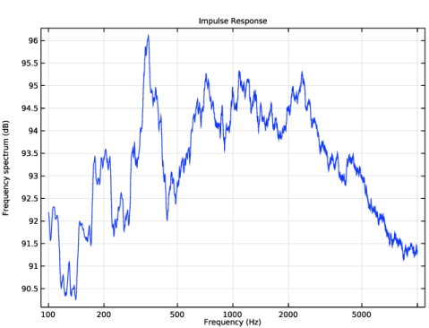
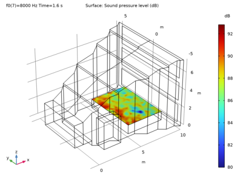
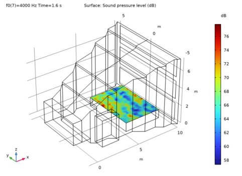
In the Settings window for Surface, click Replace Expression in the upper-right corner of the Expression section. From the menu, choose Component 1 (comp1)>Ray Acoustics>Accumulated variables>Wall intensity comp1.rac.wall8.spl1.Iw>rac.wall8.spl1.Lp - Sound pressure level - dB.
|
|
3
|
|
4
|
|
1
|
|
2
|
|
3
|
|
4
|
|
5
|
|
6
|
|
7
|
|
8
|
|
1
|
|
2
|
|
3
|
|
4
|
|
5
|
Click to expand the Coloring and Style section. Find the Line style subsection. From the Line list, choose None.
|
|
6
|
|
7
|
|
8
|
|
1
|
|
2
|
|
3
|
|
4
|
Locate the Legends section. In the table, enter the following settings:
|
|
5
|
|
1
|
|
2
|
|
3
|
Locate the Data section. From the Dataset list, choose Study 1 - Omnidirectional Source/Parametric Solutions 1 (sol2).
|
|
4
|
|
5
|
|
6
|
|
7
|
|
8
|
|
9
|
|
10
|
|
11
|
|
12
|
|
13
|
|
14
|
|
1
|
|
2
|
|
4
|
|
5
|
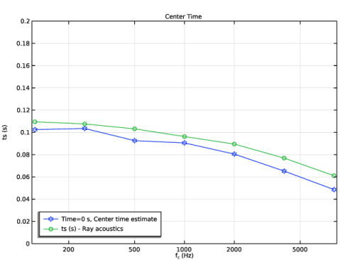
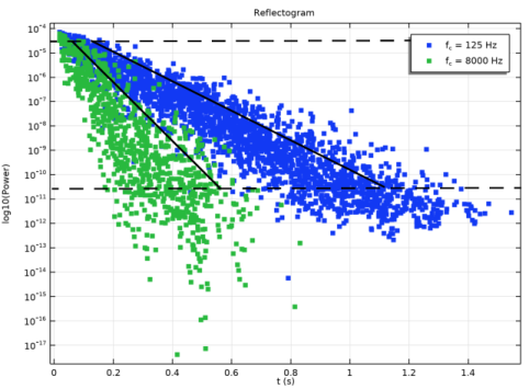
Click to expand the Coloring and Style section. Find the Line markers subsection. From the Marker list, choose Star.
|
|
1
|
|
2
|
|
3
|
|
4
|
|
5
|
|
6
|
Locate the Coloring and Style section. Find the Line markers subsection. From the Marker list, choose Circle.
|
|
7
|
|
8
|
|
9
|
|
1
|
|
2
|
|
3
|
Locate the Data section. From the Dataset list, choose Study 1 - Omnidirectional Source/Parametric Solutions 1 (sol2).
|
|
4
|
|
5
|
|
6
|
|
7
|
|
8
|
|
9
|
|
10
|
|
11
|
|
12
|
|
13
|
|
14
|
|
15
|
|
1
|
|
2
|
|
4
|
|
5
|
Click to expand the Coloring and Style section. Find the Line markers subsection. From the Marker list, choose Star.
|
|
1
|
|
2
|
|
3
|
|
4
|
|
5
|
|
6
|
Locate the Coloring and Style section. Find the Line markers subsection. From the Marker list, choose Circle.
|
|
7
|
|
8
|
|
9
|
|
1
|
|
2
|
|
3
|
|
4
|
|
5
|
|
6
|
|
7
|
|
1
|
|
2
|
|
1
|
|
2
|
|
3
|
|
4
|
|
1
|
|
2
|
|
3
|
|
4
|
|
5
|
|
6
|
|
7
|
|
8
|
|
1
|
|
2
|
|
1
|
|
2
|
|
3
|
|
4
|
|
1
|
|
2
|
|
3
|
|
4
|
|
5
|
|
6
|
|
7
|
|
1
|
|
2
|
|
1
|
|
2
|
|
3
|
|
4
|
|
1
|
|
2
|
|
3
|
|
4
|
|
5
|
|
6
|
|
7
|
|
8
|
|
1
|
|
2
|
|
3
|
|
4
|
|
1
|
In the Model Builder window, under Results, Ctrl-click to select Definition, Clarity, Center Time, Reverberation Times, and Speech Transmission Index.
|
|
2
|
Right-click and choose Group.
|
|
1
|
|
2
|
|
3
|
Find the Studies subsection. In the Select Study tree, select Preset Studies for Selected Physics Interfaces>Ray Tracing.
|
|
4
|
|
5
|
|
1
|
|
2
|
|
1
|
|
2
|
|
3
|
|
4
|
|
5
|
Locate the Physics and Variables Selection section. Select the Modify model configuration for study step check box.
|
|
6
|
|
7
|
Click
|
|
1
|
|
2
|
|
3
|
Click
|
|
6
|
Click
|
|
7
|
|
8
|
|
9
|
|
10
|
Click Replace.
|
|
11
|
|
1
|
|
2
|
|
3
|
|
1
|
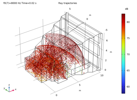
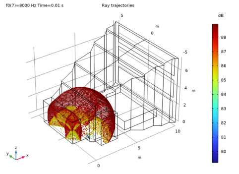
In the Model Builder window, expand the Ray Trajectories (rac) 1 node, then click Ray Trajectories 1.
|
|
2
|
|
3
|
|
4
|
|
1
|
|
2
|
|
3
|
|
4
|
|
1
|
|
2
|
|
3
|
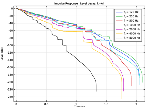
Locate the Data section. From the Dataset list, choose Study 2 - Directional Loudspeaker/Solution 10 (sol10).
|
|
4
|
|
1
|
|
2
|
|
3
|
|
4
|
|
5
|
|
6
|
|
1
|
|
2
|
|
3
|
|
4
|
|
1
|
|
2
|
|
3
|
Click
|
|
4
|
Browse to the model’s Application Libraries folder and double-click the file small_concert_hall.mphbin.
|
|
5
|
Click
|
|
6
|
|
1
|
|
2
|
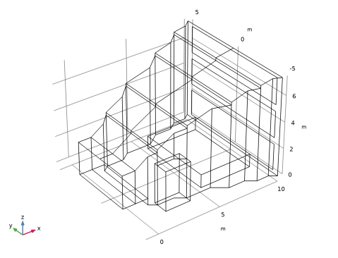
On the object imp1, select Boundary 40 only.
|
|
1
|
|
2
|
On the object del1, select Boundary 39 only.
|
|
3
|
|
4
|
|
5
|
|
1
|
|
2
|
On the object ext1, select Boundary 41 only.
|
|
1
|
|
2
|
|
3
|
|
4
|
On the object del2, select Boundaries 63–65 only.
|
|
1
|
|
2
|
|
3
|
|
4
|
On the object del2, select Boundaries 39–42 and 59 only.
|
|
1
|
|
2
|
|
3
|
|
4
|
On the object del2, select Boundaries 13, 15, 29, 30, 43, 44, 51, and 52 only.
|
|
1
|
|
2
|
|
3
|
|
4
|
On the object del2, select Boundaries 3, 8, 12, 14, 18, and 21 only.
|
|
1
|
|
2
|
|
3
|
|
4
|
On the object del2, select Boundaries 16, 19, 20, 23, 31, and 32 only.
|
|
1
|
|
2
|
|
3
|
|
4
|
On the object del2, select Boundaries 1, 2, 4–7, 9–11, 17, 22, 24–28, 34–37, 45–50, 53–58, and 60–62 only.
|
|
1
|
|
2
|
|
3
|
|
4
|
On the object del2, select Boundaries 33 and 38 only.
|
|
1
|
|
2
|