PDF

Generation of Lamb Waves for Nondestructive Inspection of Plate Specimens
Introduction
Lamb waves are named after Horace Lamb who studied the motion of two-dimensional waves in solids bounded by two parallel planes in his classic work Ref. 1. He obtained two sets of analytical solutions for symmetric and antisymmetric modes propagating in infinite plates with a finite thickness. Lamb waves belong to guided waves that propagate in long solid objects (waveguides), such as rods; plates; or pipes, but also in more complex structures, like rails, where it is impossible to find an analytical solution.
Numerical modeling of Lamb waves is essential for the analysis and design of the structural health monitoring (SHM) systems for long range ultrasonic testing. The design of an SHM system based on guided waves consists of two main parts. In the first place, it is required to know the dispersion curves for the modes that can propagate in the waveguide of a certain cross section. In the second place, the propagation of a chosen mode through the waveguide and its reflection from a possible irregularity in the cross-section area (a fracture or a corrosion defect) is analyzed in the time domain.
This tutorial studies the propagation of guided waves in a steel plate with a finite width and thickness. In the first part, the Mode Analysis study for the Solid Mechanics physics interface applied on the 2D cross section of the plate computes the propagating modes. This approach is also sometimes referred to as the semi-analytical finite element (SAFE) method. In the second part, an angle beam wedge excites the desired mode in the plate with a flaw, which is modeled in 3D using the Elastic Wave, Time Explicit physics interface.
Model Definition
The steel plate used here is 15 mm wide and 5 mm thick. An angle beam wedge transducer placed on top of the plate generates the antisymmetric or flexural zero-order mode (A0) in the plate. The wedge is made of plastic and has the angle of incidence of 70°. A normal velocity applied on the excitation area of the wedge generates a longitudinal wave that travels through the wedge. The setup is shown in Figure 1. This tutorial thus omits the details on the transducer modeling which are, for example, given in Angle Beam Nondestructive Testing tutorial model.
The source signal is a five-cycle tone burst with the center frequency f0 = 200 kHz as shown in Figure 2. The longitudinal wave velocity in plastic is cp = 2080 m/s and the estimated velocity (see the next section) of the refracted A0-mode in the plate at the chosen frequency is vLamb = 2300 m/s. The wave refraction is computed according to Snell’s law as
(1)
The refraction angle β = 90°, which yields the critical angle of about α = 65°. Since the angle of incident of the chosen wedge is larger than the critical angle, the wave sent through the wedge will be refracted into the desired mode in the plate.
Figure 1: Model setup including wedge and test plate.
The plate has a flaw, which is a fracture with the dimensions of the plate thickness and half of its width. The orientation of the fracture makes the guided wave hit it at a right angle. Part of the wave will pass further along the plate, and part of it will be reflected back to the wedge. The transmitted and reflected signals are recorded at four observation points placed on the top surface of the plate at equal distance before and after the fracture.
Figure 2: Five-cycle tone burst source signal.
Results and Discussion
First, look at the dispersion diagrams, Figure 3 and Figure 4, obtained from the mode analysis for the plate cross section. The plots show the out-of-plane wave numbers, kn, and the phase velocities, vp, of the propagating modes, respectively. The phase velocities are defined as
and the group velocities as
Note that the phase velocities in Figure 4 are normalized to the shear wave speed in steel. The red lines depict the wave numbers and normalized velocities of the pure longitudinal and shear waves in steel.
Figure 3 and Figure 4 indicate that each propagating mode exists above a certain nascent frequency (cut on/off frequency of the mode). Four of the computed modes have nascent frequencies of zero and thus exist throughout the whole frequency range. The number of such modes in this example is higher than that from the classic result of Lamb (two zero-order antisymmetric, A0, and symmetric, S0, modes), which is due to the finite (and comparable) dimensions of the plate cross section. The more complex the waveguide cross section, the higher number of modes will be able to propagate in it.
Figure 3: Dispersion curves of Lamb waves in the plate: out-of-plane wave number.
The lowermost curve in Figure 4 corresponds to the vertically polarized A0-mode: its vertical displacements are symmetric while the out-of-plane ones are antisymmetric (see the orientation of the coordinate axes in Figure 1). It is the slowest propagating mode in the plate and is depicted in the upper-left corner in Figure 5. Figure 5 shows the profiles of the modes propagating at f0 = 200 kHz that are symmetric with respect to the sagittal plane of the system, as those are the only ones that can be excited by the current design of the wedge.
Figure 4 exhibits the known property of Lamb waves: they are dispersive, that is, their speed depends on the frequency. In this regards, the choice of the excitation frequency is no accident For example, the estimated velocity of the A0-mode at 100 kHz is about 1720 m/s. This value is less than the longitudinal wave speed in the wedge, thus making the desired wave refraction unreachable (see Equation 1) for the current dimension of the plate and the wedge material, and the angle of incidence.
Figure 4: Dispersion curves of Lamb waves in the plate: normalized phase velocity.
The second part of this tutorial is dedicated to the analysis of the selected mode propagation in the 3D plate and its reflection from the flaw. The evolution of the traveling wave is illustrated in Figure 6. Note that Figure 6 shows the velocity magnitude profiles only in the plate, as those in the wedge are of no interest here.
The wave packet travels toward the defect (t = 80 μs) until it hits it (t = 110 μs). Then a portion of the packet passes further down the plate while another portion is reflected back to the wedge (t = 140 μs). The reflected part of the signal travels back toward the wedge (t = 170 μs). Note that the signal is no longer symmetric with respect to the sagittal plane after it has hit the flaw.
The vertical displacements of the signal computed at the listening points placed before and after the fracture are depicted in Figure 7 on the left and on the right, respectively. The blue lines correspond to the side of the plate with the fracture; the green lines, to the opposite side. As the wave is dispersive, the wave packet travels with the group velocity. Measuring the time delay between the incident and reflected waves yields the group velocity of 3153 m/s. The group velocity of the A0-mode estimated from the dispersion diagram is about 3130 m/s, which is close to one computed from the 3D time-domain analysis.
Figure 5: Profiles of the modes propagating at f0 = 200 kHz and symmetric with respect to the sagittal plane.
The A0-mode is clearly visible when it propagates in the plate, especially at the times before it has reached the flaw. Although this mode has the highest magnitude, it is not the only refracted wave that is exited by the transducer. The other mode is faster than the A0-mode and is vaguely seen in Figure 6 at t = 80 μs. Its distinct shape is available from Figure 8 that shows the vertical (y-component) and longitudinal (z-component) velocity components on the top and the bottom of the plate at t = 80 μs. The vertical velocity of the slower A0-mode is in phase on the top and the bottom of the plate, while that of the faster mode is 180° out of phase. The opposite applies to the longitudinal velocity. The faster mode propagating in the plate is the one depicted in the lower-left corner in Figure 5. It has the phase velocity of 5435 m/s, and its nascent frequency lies between 160 and 170 kHz as seen from Figure 4.
Figure 6: Wave profiles at t = 80, 110, 140, and 170 μs.
Figure 7: Vertical displacements at the listening points before (left) and after (right) the defect.
Figure 8: Velocity profiles on the top (green) and the bottom (blue) of the plate at t = 80 μs.
Reference
1. H. Lamb, “On waves in an elastic plate,” Proc. R. Soc. Lond. A, vol. 93, issue 648, 1917.
Application Library path: Acoustics_Module/Ultrasound/lamb_waves_ndt_plate
Modeling Instructions
From the File menu, choose New.
New
In the New window, click  Blank Model.
Global Definitions
Parameters: Geometrical Parameters
1
In the Model Builder window, under Global Definitions click Parameters 1.
2
In the Settings window for Parameters, locate the Parameters section.
3
Click  Load from File.
4
5
In the Label text field, type Parameters: Geometrical Parameters.
Parameters: Model Parameters
1
In the Home toolbar, click  Parameters and choose Add>Parameters.
2
In the Settings window for Parameters, locate the Parameters section.
3
Click  Load from File.
4
5
In the Label text field, type Parameters: Model Parameters.
Steel
1
In the Model Builder window, under Global Definitions right-click Materials and choose Blank Material.
2
In the Settings window for Material, type Steel in the Label text field.
3
Locate the Material Properties section. In the Material properties tree, select Basic Properties>Density.
4
Click  Add to Material.
5
Locate the Material Contents section. In the table, enter the following settings:
6
Locate the Material Properties section. In the Material properties tree, select Solid Mechanics>Linear Elastic Material>Pressure-Wave and Shear-Wave Speeds.
7
Click  Add to Material.
8
Locate the Material Contents section. In the table, enter the following settings:
Plastic
1
Right-click Materials and choose Blank Material.
2
In the Settings window for Material, type Plastic in the Label text field.
3
Locate the Material Properties section. In the Material properties tree, select Basic Properties>Density.
4
Click  Add to Material.
5
Locate the Material Contents section. In the table, enter the following settings:
6
Locate the Material Properties section. In the Material properties tree, select Solid Mechanics>Linear Elastic Material>Pressure-Wave and Shear-Wave Speeds.
7
Click  Add to Material.
8
Locate the Material Contents section. In the table, enter the following settings:
First, compute the modes that can propagate in the waveguide of a rectangular cross section.
Add Component
In the Home toolbar, click  Add Component and choose 2D.
Geometry 1
Rectangle 1 (r1)
1
In the Geometry toolbar, click  Rectangle.
2
In the Settings window for Rectangle, locate the Size and Shape section.
3
In the Width text field, type W_plate.
4
In the Height text field, type D_plate.
5
Locate the Position section. From the Base list, choose Center.
6
Click  Build All Objects.
Materials
Steel
1
In the Model Builder window, under Component 1 (comp1) right-click Materials and choose More Materials>Material Link.
2
In the Settings window for Material Link, type Steel in the Label text field.
Component 1 (comp1)
In the Home toolbar, click  Windows and choose Add Physics.
Add Physics
1
Go to the Add Physics window.
2
In the tree, select Structural Mechanics>Solid Mechanics (solid).
3
Click Add to Component 1 in the window toolbar.
Solid Mechanics (solid)
In the Home toolbar, click  Windows and choose Add Physics.
Linear Elastic Material 1
1
In the Model Builder window, under Component 1 (comp1)>Solid Mechanics (solid) click Linear Elastic Material 1.
2
In the Settings window for Linear Elastic Material, locate the Linear Elastic Material section.
3
From the Specify list, choose Pressure-wave and shear-wave speeds.
Mesh 1
Mapped 1
In the Mesh toolbar, click  Mapped.
Size
1
In the Model Builder window, click Size.
2
In the Settings window for Size, locate the Element Size section.
3
From the Predefined list, choose Extra fine.
4
Click  Build All.
Results
1
In the Model Builder window, click Results.
2
In the Settings window for Results, locate the Update of Results section.
3
Select the Only plot when requested check box.
4
Locate the Save Data in the Model section. From the Save plot data list, choose On.
Root
In the Home toolbar, click  Windows and choose Add Study.
Add Study
1
Go to the Add Study window.
2
Find the Studies subsection. In the Select Study tree, select Preset Studies for Selected Physics Interfaces>Mode Analysis.
3
Click Add Study in the window toolbar.
Study 1 - Mode Analysis
1
In the Model Builder window, click Study 1.
2
In the Settings window for Study, type Study 1 - Mode Analysis in the Label text field.
3
Locate the Study Settings section. Clear the Generate default plots check box.
Step 1: Mode Analysis
1
In the Model Builder window, under Study 1 - Mode Analysis click Step 1: Mode Analysis.
2
In the Settings window for Mode Analysis, locate the Study Settings section.
3
In the Mode analysis frequency text field, type f0.
4
Select the Desired number of modes check box. In the associated text field, type 20.
5
Find the Search region subsection. In the Unit field, type 1/m.
6
Select the Search for modes around check box. In the associated text field, type ks.
Search for the modes within the frequency range from 0 to fmax.
Parametric Sweep
1
In the Study toolbar, click  Parametric Sweep.
2
In the Settings window for Parametric Sweep, locate the Study Settings section.
3
4
5
In the Study toolbar, click  Compute.
Results
Dispersion Curves, Phase Velocity
1
In the Home toolbar, click  Add Plot Group and choose 1D Plot Group.
2
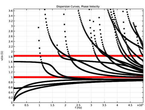
In the Settings window for 1D Plot Group, type Dispersion Curves, Phase Velocity in the Label text field.
3
Locate the Data section. From the Dataset list, choose Study 1 - Mode Analysis/Parametric Solutions 1 (sol2).
4
Click to expand the Title section. From the Title type list, choose Label.
5
Locate the Plot Settings section.
6
Select the x-axis label check box. In the associated text field, type f (Hz).
7
Select the y-axis label check box. In the associated text field, type v/cs (1).
8
Locate the Axis section. Select the Manual axis limits check box.
9
In the x minimum text field, type 0.
10
In the x maximum text field, type fmax.
11
In the y minimum text field, type 0.
12
In the y maximum text field, type 2*cp_steel/cs_steel.
13
Locate the Legend section. Clear the Show legends check box.
Global 1
1
Right-click Dispersion Curves, Phase Velocity and choose Global.
2
In the Settings window for Global, locate the Data section.
3
From the Dataset list, choose Study 1 - Mode Analysis/Parametric Solutions 1 (sol2).
4
From the Out-of-plane wave number selection list, choose First.
5
Locate the y-Axis Data section. In the table, enter the following settings:
6
Locate the x-Axis Data section. From the Parameter list, choose Expression.
7
In the Expression text field, type f0.
8
Click to expand the Coloring and Style section. Find the Line style subsection. From the Line list, choose None.
9
From the Color list, choose Red.
10
Find the Line markers subsection. From the Marker list, choose Circle.
Global 2
1
In the Model Builder window, right-click Dispersion Curves, Phase Velocity and choose Global.
2
In the Settings window for Global, locate the y-Axis Data section.
3
4
Locate the x-Axis Data section. From the Parameter list, choose Expression.
5
In the Expression text field, type f0.
6
Locate the Coloring and Style section. Find the Line style subsection. From the Line list, choose None.
7
From the Color list, choose Black.
8
Find the Line markers subsection. From the Marker list, choose Point.
Plot the dispersion curves for the modes that propagate in the out-of-plane direction. The wave numbers of such modes will have their imaginary parts close to 0. Plot the curves that lie in the upper half plane.
Filter 1
1
Right-click Global 2 and choose Filter.
2
In the Settings window for Filter, locate the Point Selection section.
3
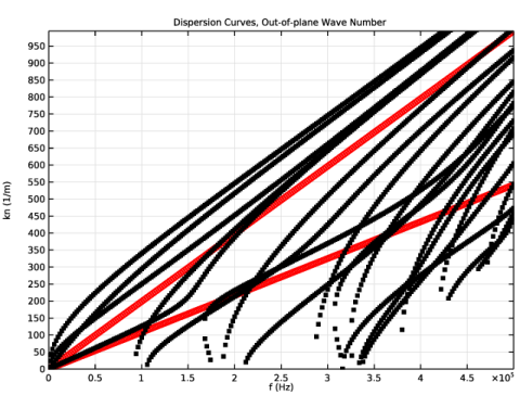
In the Logical expression for inclusion text field, type (abs(imag(solid.kn))<1)&&(real(solid.kn)>0).
4
In the Dispersion Curves, Phase Velocity toolbar, click  Plot.
Dispersion Curves, Out-of-plane Wave Number
1
In the Model Builder window, right-click Dispersion Curves, Phase Velocity and choose Duplicate.
2
In the Settings window for 1D Plot Group, type Dispersion Curves, Out-of-plane Wave Number in the Label text field.
3
Locate the Plot Settings section. In the y-axis label text field, type kn (1/m).
4
Locate the Axis section. In the y maximum text field, type omegamax/cs_steel.
Global 1
1
In the Model Builder window, expand the Dispersion Curves, Out-of-plane Wave Number node, then click Global 1.
2
In the Settings window for Global, locate the y-Axis Data section.
3
Global 2
1
In the Model Builder window, click Global 2.
2
In the Settings window for Global, locate the y-Axis Data section.
3
4
In the Dispersion Curves, Out-of-plane Wave Number toolbar, click  Plot.
Create an Extrusion 2D dataset to visualize the shapes of the modes propagating in the out-of-plane direction.
Extrusion 2D 1
1
In the Results toolbar, click  More Datasets and choose Extrusion 2D.
2
In the Settings window for Extrusion 2D, locate the Data section.
3
From the Dataset list, choose Study 1 - Mode Analysis/Parametric Solutions 1 (sol2).
4
Locate the Extrusion section. In the z maximum text field, type 10[cm].
5
In the Resolution text field, type 100.
6
Click to expand the Advanced section. In the Out-of-plane wave number text field, type solid.kn.
Mode Shape
1
In the Results toolbar, click  3D Plot Group.
2
In the Settings window for 3D Plot Group, type Mode Shape in the Label text field.
3
Locate the Data section. From the Parameter value (f0 (Hz)) list, choose 2E5.
4
From the Out-of-plane wave number (1/m) list, choose 546.38.
5
Click to expand the Title section. From the Title type list, choose Manual.
6
In the Parameter indicator text field, type kn = eval(real(solid.kn)) [1/m], v/cs = eval(omega0/real(solid.kn)/cs_steel).
Surface 1
1
Right-click Mode Shape and choose Surface.
2
In the Settings window for Surface, locate the Coloring and Style section.
3
Click  Change Color Table.
4
In the Color Table dialog box, select Rainbow>Prism in the tree.
5
Deformation 1
Right-click Surface 1 and choose Deformation.
Now, proceed to modeling of the selected mode propagation in the 3D plate.
Add Component
In the Model Builder window, right-click the root node and choose Add Component>3D.
Geometry 2
1
In the Geometry toolbar, click Insert Sequence and choose Insert Sequence.
2
3
In the Geometry toolbar, click  Build All.
Create a five-cycle tone burst source signal.
Definitions (comp2)
Rectangle 1 (rect1)
1
In the Home toolbar, click  Functions and choose Local>Rectangle.
2
In the Settings window for Rectangle, locate the Parameters section.
3
In the Lower limit text field, type 0.
4
In the Upper limit text field, type 4*T0.
5
Click to expand the Smoothing section. Clear the Size of transition zone check box.
Normal Velocity Source
1
In the Home toolbar, click  Functions and choose Local>Analytic.
2
In the Settings window for Analytic, type Normal Velocity Source in the Label text field.
3
In the Function name text field, type vn.
4
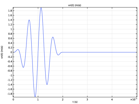
Locate the Definition section. In the Expression text field, type sin(omega0*t)*(1 - cos(omega0*t/4))*rect1(t).
5
In the Arguments text field, type t.
6
Locate the Units section. In the Function text field, type m/s.
7
8
Locate the Plot Parameters section. In the table, enter the following settings:
9
Wedge
1
In the Definitions toolbar, click  Explicit.
2
In the Settings window for Explicit, type Wedge in the Label text field.
3
Plate
1
In the Definitions toolbar, click  Explicit.
2
In the Settings window for Explicit, type Plate in the Label text field.
3
AL
1
In the Definitions toolbar, click  Explicit.
2
In the Settings window for Explicit, type AL in the Label text field.
3
Probes
1
In the Definitions toolbar, click  Explicit.
2
In the Settings window for Explicit, locate the Input Entities section.
3
From the Geometric entity level list, choose Point.
4
5
In the Label text field, type Probes.
Exterior Boundaires
1
In the Definitions toolbar, click  Adjacent.
2
In the Settings window for Adjacent, type Exterior Boundaires in the Label text field.
3
Locate the Input Entities section. Under Input selections, click  Add.
4
In the Add dialog box, in the Input selections list, choose Wedge and Plate.
5
Identity Boundary Pair 1 (p1)
1
In the Definitions toolbar, click  Pairs and choose Identity Boundary Pair.
2
3
In the Settings window for Pair, locate the Destination Boundaries section.
4
Click to select the  Activate Selection toggle button.
5
Materials
Steel
1
In the Model Builder window, under Component 2 (comp2) right-click Materials and choose More Materials>Material Link.
2
In the Settings window for Material Link, locate the Geometric Entity Selection section.
3
From the Selection list, choose Plate.
4
In the Label text field, type Steel.
Plastic
1
Right-click Materials and choose More Materials>Material Link.
2
In the Settings window for Material Link, locate the Geometric Entity Selection section.
3
From the Selection list, choose Wedge.
4
Locate the Link Settings section. From the Material list, choose Plastic (mat2).
5
In the Label text field, type Plastic.
Component 2 (comp2)
In the Home toolbar, click  Windows and choose Add Physics.
Add Physics
1
Go to the Add Physics window.
2
In the tree, select Acoustics>Elastic Waves>Elastic Waves, Time Explicit (elte).
3
Click Add to Component 2 in the window toolbar.
4
Find the Physics interfaces in study subsection. In the table, clear the Solve check box for Study 1 - Mode Analysis.
Elastic Waves, Time Explicit (elte)
Elastic Waves, Time Explicit Model 1
In the Model Builder window, under Component 2 (comp2)>Elastic Waves, Time Explicit (elte) click Elastic Waves, Time Explicit Model 1.
Compute Displacement 1
1
In the Physics toolbar, click  Attributes and choose Compute Displacement.
2
In the Settings window for Compute Displacement, locate the Point Selection section.
3
From the Selection list, choose Probes.
Prescribed Velocity 1
1
In the Physics toolbar, click  Boundaries and choose Prescribed Velocity.
2
3
In the Settings window for Prescribed Velocity, locate the Coordinate System Selection section.
4
From the Coordinate system list, choose Boundary System 2 (sys2).
5
Locate the Prescribed Velocity section. Specify the v0 vector as
Low-Reflecting Boundary 1
1
In the Physics toolbar, click  Boundaries and choose Low-Reflecting Boundary.
2
Fracture 1
1
In the Physics toolbar, click  Boundaries and choose Fracture.
2
Create four domain probe points along the wave propagation path (two before and two after the defect) where the vertical displacements will be recorded.
Definitions (comp2)
Point Probe 1 (point1)
1
In the Definitions toolbar, click  Probes and choose Point Probe.
2
In the Settings window for Point Probe, locate the Source Selection section.
3
Click  Clear Selection.
4
5
Locate the Expression section. In the Expression text field, type elte.uy.
6
Select the Description check box. In the associated text field, type uy.
Point Probe 2 (point2)
1
Right-click Point Probe 1 (point1) and choose Duplicate.
2
Point Probe 3 (point3)
1
Right-click Point Probe 2 (point2) and choose Duplicate.
2
In the Settings window for Point Probe, locate the Source Selection section.
3
Click  Clear Selection.
4
Point Probe 4 (point4)
1
Right-click Point Probe 3 (point3) and choose Duplicate.
2
In the Settings window for Point Probe, locate the Source Selection section.
3
Click  Clear Selection.
4
Point Probe 1 (point1), Point Probe 2 (point2), Point Probe 3 (point3), Point Probe 4 (point4)
1
In the Model Builder window, under Component 2 (comp2)>Definitions, Ctrl-click to select Point Probe 1 (point1), Point Probe 2 (point2), Point Probe 3 (point3), and Point Probe 4 (point4).
2
y-displacement
In the Settings window for Group, type y-displacement in the Label text field.
Absorbing Layer 1 (ab1)
1
In the Definitions toolbar, click  Absorbing Layer.
2
In the Settings window for Absorbing Layer, locate the Domain Selection section.
3
From the Selection list, choose AL.
Mesh 2
Mapped 1
1
In the Mesh toolbar, click  Boundary and choose Mapped.
2
Swept 1
1
In the Mesh toolbar, click  Swept.
2
In the Settings window for Swept, locate the Domain Selection section.
3
From the Geometric entity level list, choose Domain.
4
From the Selection list, choose Plate.
Size
1
In the Model Builder window, click Size.
2
In the Settings window for Size, locate the Element Size section.
3
Click the Custom button.
4
Locate the Element Size Parameters section. In the Maximum element size text field, type v_lamb/(1.5*2*f0).
Free Tetrahedral 1
In the Mesh toolbar, click  Free Tetrahedral.
Size 1
1
Right-click Free Tetrahedral 1 and choose Size.
2
In the Settings window for Size, locate the Element Size section.
3
Click the Custom button.
4
Locate the Element Size Parameters section.
5
Select the Maximum element size check box. In the associated text field, type cp_plast/(1.5*2*f0).
Free Tetrahedral 1
1
In the Model Builder window, click Free Tetrahedral 1.
2
In the Settings window for Free Tetrahedral, click to expand the Element Quality Optimization section.
3
From the Optimization level list, choose High.
4
Select the Avoid too small elements check box.
5
Click  Build All.
Root
In the Home toolbar, click  Windows and choose Add Study.
Add Study
1
Go to the Add Study window.
2
Find the Physics interfaces in study subsection. In the table, clear the Solve check box for Solid Mechanics (solid).
3
Find the Studies subsection. In the Select Study tree, select General Studies>Time Dependent.
4
Click Add Study in the window toolbar.
Study 2 - Wave Propagation
1
In the Model Builder window, click Study 2.
2
In the Settings window for Study, type Study 2 - Wave Propagation in the Label text field.
Step 1: Time Dependent
1
In the Model Builder window, under Study 2 - Wave Propagation click Step 1: Time Dependent.
2
In the Settings window for Time Dependent, locate the Study Settings section.
3
In the Output times text field, type range(0, T0, 45*T0).
4
Click to expand the Values of Dependent Variables section. Find the Store fields in output subsection. From the Settings list, choose For selections.
5
Under Selections, click  Add.
6
In the Add dialog box, select Exterior Boundaires in the Selections list.
7
8
In the Home toolbar, click  Compute.
Results
Surface 1
In the Model Builder window, expand the Results>Velocity Magnitude (elte) node, then click Surface 1.
Selection 1
1
Right-click Surface 1 and choose Selection.
2
In the Settings window for Selection, locate the Selection section.
3
From the Geometric entity level list, choose Domain.
4
From the Selection list, choose Plate.
Surface 1
1
In the Model Builder window, click Surface 1.
2
In the Settings window for Surface, locate the Coloring and Style section.
3
Click  Change Color Table.
4
In the Color Table dialog box, select Rainbow>Prism in the tree.
5
Probe Plot Displacements
1
In the Model Builder window, under Results click Probe Plot Group 6.
2
In the Settings window for 1D Plot Group, type Probe Plot Displacements in the Label text field.
3
Locate the Plot Settings section.
4
Select the y-axis label check box. In the associated text field, type Vertical displacement (m).
5
Locate the Legend section. From the Layout list, choose Outside graph axis area.
6
From the Position list, choose Bottom.
7
In the Number of rows text field, type 2.
Probe Table Graph 1
1
In the Model Builder window, expand the Probe Plot Displacements node, then click Probe Table Graph 1.
2
In the Settings window for Table Graph, locate the Data section.
3
In the Columns list, choose uy (m), Point Probe 3 and uy (m), Point Probe 4.
4
In the Columns list, choose uy (m), Point Probe 1 and uy (m), Point Probe 2.
Velocity, y-component
1
In the Home toolbar, click  Add Plot Group and choose 1D Plot Group.
2
In the Settings window for 1D Plot Group, type Velocity, y-component in the Label text field.
3
Locate the Data section. From the Dataset list, choose Study 2 - Wave Propagation/Solution 253 (4) (sol253).
4
From the Time selection list, choose From list.
5
In the Times (s) list, select 8E-5.
6
Locate the Title section. From the Title type list, choose Label.
Line Graph 1
1
Right-click Velocity, y-component and choose Line Graph.
2
3
In the Settings window for Line Graph, locate the y-Axis Data section.
4
In the Expression text field, type v2y.
5
Locate the x-Axis Data section. From the Parameter list, choose Expression.
6
In the Expression text field, type z.
7
Click to expand the Legends section. Select the Show legends check box.
8
From the Legends list, choose Manual.
9
Line Graph 2
1
Right-click Line Graph 1 and choose Duplicate.
2
In the Settings window for Line Graph, locate the Selection section.
3
Click  Clear Selection.
4
5
Locate the Legends section. In the table, enter the following settings:
6
In the Velocity, y-component toolbar, click  Plot.
 
Appendix — Geometry Modeling Instructions
From the File menu, choose New.
New
In the New window, click  Model Wizard.
Model Wizard
1
In the Model Wizard window, click  3D.
2
Global Definitions
Geometry Parameters
1
In the Model Builder window, under Global Definitions click Parameters 1.
2
In the Settings window for Parameters, locate the Parameters section.
3
Click  Load from File.
4
5
In the Label text field, type Geometry Parameters.
Geometry 1
Work Plane 1 (wp1)
In the Geometry toolbar, click  Work Plane.
Work Plane 1 (wp1)>Plane Geometry
In the Model Builder window, click Plane Geometry.
Work Plane 1 (wp1)>Rectangle 1 (r1)
1
In the Work Plane toolbar, click  Rectangle.
2
In the Settings window for Rectangle, locate the Size and Shape section.
3
In the Width text field, type W_plate.
4
In the Height text field, type D_plate.
5
Locate the Position section. From the Base list, choose Center.
Extrude 1 (ext1)
1
In the Model Builder window, right-click Geometry 1 and choose Extrude.
2
In the Settings window for Extrude, locate the Distances section.
3
Move 1 (mov1)
1
In the Geometry toolbar, click  Transforms and choose Move.
2
3
In the Settings window for Move, locate the Displacement section.
4
In the x text field, type W_plate/2.
5
In the y text field, type -D_plate/2.
6
In the z text field, type -L_plate/4.
Block 1 (blk1)
1
In the Geometry toolbar, click  Block.
2
In the Settings window for Block, locate the Size and Shape section.
3
In the Width text field, type W_wedge.
4
In the Depth text field, type H_wedge.
5
In the Height text field, type L_wedge.
6
Locate the Position section. In the x text field, type (W_plate - W_wedge)/2.
Work Plane 2 (wp2)
1
In the Geometry toolbar, click  Work Plane.
2
In the Settings window for Work Plane, locate the Plane Definition section.
3
From the Plane type list, choose Normal vector.
4
Find the Normal vector subsection. In the y text field, type cos(alpha).
5
In the z text field, type -sin(alpha).
6
Find the Point on plane subsection. In the y text field, type H_wedge - L_slope*sin(alpha).
Work Plane 2 (wp2)>Plane Geometry
In the Model Builder window, click Plane Geometry.
Work Plane 2 (wp2)>Circle 1 (c1)
1
In the Work Plane toolbar, click  Circle.
2
In the Settings window for Circle, locate the Size and Shape section.
3
In the Radius text field, type R_source.
4
Locate the Position section. In the xw text field, type -L_slope*sin(alpha)/2.
5
In the yw text field, type -W_plate/2.
Partition Objects 1 (par1)
1
In the Model Builder window, right-click Geometry 1 and choose Booleans and Partitions>Partition Objects.
2
3
In the Settings window for Partition Objects, locate the Partition Objects section.
4
From the Partition with list, choose Work plane.
Delete Entities 1 (del1)
1
Right-click Geometry 1 and choose Delete Entities.
2
In the Settings window for Delete Entities, locate the Entities or Objects to Delete section.
3
From the Geometric entity level list, choose Domain.
4
On the object par1, select Domain 2 only.
Parametric Surface 1 (ps1)
1
In the Geometry toolbar, click  More Primitives and choose Parametric Surface.
2
In the Settings window for Parametric Surface, locate the Parameters section.
3
Find the First parameter subsection. In the Minimum text field, type W_plate/2.
4
In the Maximum text field, type W_plate.
5
Find the Second parameter subsection. In the Minimum text field, type -D_plate.
6
In the Maximum text field, type 0.
7
Locate the Expressions section. In the x text field, type s1.
8
In the y text field, type s2.
9
In the z text field, type 0.3.
10
Click  Build Selected.
Point 1 (pt1)
1
In the Geometry toolbar, click  More Primitives and choose Point.
2
In the Settings window for Point, locate the Point section.
3
In the z text field, type 0.2.
Point 2 (pt2)
1
In the Geometry toolbar, click  More Primitives and choose Point.
2
In the Settings window for Point, locate the Point section.
3
In the z text field, type 0.4.
Copy 1 (copy1)
1
In the Geometry toolbar, click  Transforms and choose Copy.
2
Select the objects pt1 and pt2 only.
3
In the Settings window for Copy, locate the Displacement section.
4
In the x text field, type W_plate.
Union 1 (uni1)
1
In the Geometry toolbar, click  Booleans and Partitions and choose Union.
2
Select the objects copy1(1), copy1(2), mov1, ps1, pt1, and pt2 only.
Form Union (fin)
1
In the Model Builder window, under Component 1 (comp1)>Geometry 1 click Form Union (fin).
2
In the Settings window for Form Union/Assembly, locate the Form Union/Assembly section.
3
From the Action list, choose Form an assembly.
4
Clear the Create pairs check box.
5
Select the Create imprints check box.
6
Click  Build Selected.
Ignore Faces 1 (igf1)
1
In the Geometry toolbar, click  Virtual Operations and choose Ignore Faces.
2
On the object fin, select Boundary 31 only.
3
In the Geometry toolbar, click  Build All.