|
|
|
|
1
|
|
2
|
Click
|
|
1
|
|
2
|
Browse to the model’s Application Libraries folder and double-click the file angle_beam_ndt_geom_sequence.mph.
|
|
3
|
|
1
|
|
2
|
|
1
|
|
2
|
|
3
|
|
4
|
Browse to the model’s Application Libraries folder and double-click the file angle_beam_ndt_parameters.txt.
|
|
5
|
|
1
|
|
2
|
|
3
|
|
4
|
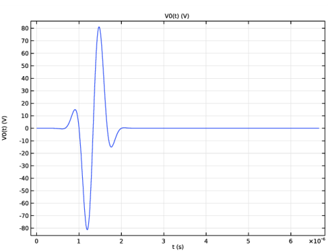
Locate the Definition section. In the Expression text field, type 100*exp(-((t - 2*T0)/(T0/2))^2)*sin(2*pi*f0*t).
|
|
5
|
|
6
|
|
8
|
|
9
|
|
1
|
|
1
|
|
2
|
|
3
|
|
4
|
Click
|
|
5
|
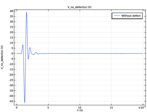
Browse to the model’s Application Libraries folder and double-click the file angle_beam_ndt_no_defect_signal.txt.
|
|
6
|
Find the Functions subsection. In the table, enter the following settings:
|
|
7
|
|
8
|
|
9
|
In the Argument table, enter the following settings:
|
|
10
|
|
1
|
|
2
|
|
3
|
|
4
|
|
6
|
|
1
|
|
3
|
|
4
|
|
1
|
|
3
|
|
4
|
|
1
|
|
3
|
|
4
|
|
1
|
|
3
|
|
4
|
|
1
|
|
3
|
|
4
|
|
1
|
|
2
|
|
3
|
|
5
|
|
6
|
|
1
|
|
2
|
|
3
|
|
1
|
|
2
|
|
3
|
|
4
|
|
5
|
|
6
|
|
7
|
Click
|
|
1
|
|
2
|
|
3
|
|
4
|
|
1
|
In the Model Builder window, under Component 1 (comp1)>Elastic Waves, Time Explicit (elte) click Elastic Waves, Time Explicit Model 1.
|
|
2
|
In the Settings window for Elastic Waves, Time Explicit Model, locate the Linear Elastic Material section.
|
|
3
|
|
1
|
|
2
|
|
3
|
|
1
|
|
1
|
|
1
|
|
2
|
|
3
|
|
4
|
|
5
|
|
6
|
|
7
|
|
8
|
|
1
|
|
2
|
|
3
|
|
1
|
|
2
|
|
3
|
|
4
|
|
5
|
|
1
|
|
2
|
|
3
|
|
4
|
|
5
|
|
1
|
In the Model Builder window, under Component 1 (comp1)>Elastic Waves, Time Explicit (elte) click Piezoelectric Material 1.
|
|
2
|
|
3
|
|
1
|
|
2
|
|
3
|
|
4
|
|
5
|
|
6
|
|
7
|
|
1
|
|
2
|
|
3
|
|
1
|
|
2
|
|
1
|
|
2
|
|
3
|
|
1
|
|
1
|
|
3
|
|
4
|
|
1
|
|
2
|
|
3
|
|
4
|
|
1
|
|
2
|
|
4
|
|
1
|
|
2
|
|
4
|
|
1
|
|
2
|
|
3
|
|
4
|
|
1
|
|
2
|
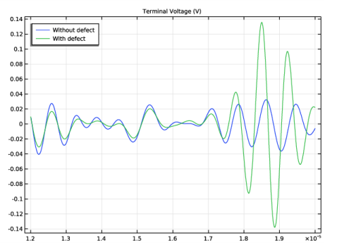
In the Settings window for Global Variable Probe, type V_with_defect in the Variable name text field.
|
|
3
|
Click Replace Expression in the upper-right corner of the Expression section. From the menu, choose Component 1 (comp1)>Electrostatics>Terminals>es.V0_1 - Terminal voltage - V.
|
|
4
|
|
5
|
|
1
|
|
1
|
|
2
|
|
3
|
In the tree, select Built-in>Aluminum.
|
|
4
|
|
5
|
|
6
|
|
1
|
|
2
|
|
1
|
|
2
|
|
3
|
|
4
|
|
1
|
|
2
|
|
1
|
|
2
|
|
3
|
|
4
|
|
5
|
|
1
|
|
2
|
|
3
|
|
4
|
|
5
|
|
1
|
|
2
|
|
3
|
|
1
|
|
3
|
|
4
|
|
1
|
|
2
|
|
3
|
|
4
|
|
5
|
|
6
|
|
1
|
|
2
|
|
3
|
|
4
|
|
5
|
|
6
|
|
1
|
|
2
|
|
3
|
|
4
|
|
5
|
|
6
|
|
7
|
|
1
|
|
2
|
|
3
|
|
4
|
|
5
|
|
6
|
|
7
|
|
1
|
|
2
|
|
3
|
|
4
|
|
5
|
|
6
|
|
7
|
|
8
|
|
1
|
|
2
|
|
3
|
|
4
|
|
5
|
|
1
|
|
2
|
|
3
|
|
1
|
|
2
|
|
3
|
|
1
|
|
2
|
|
3
|
|
4
|
|
6
|
|
1
|
|
2
|
|
3
|
|
1
|
|
2
|
|
3
|
|
4
|
|
5
|
|
6
|
Click OK.
|
|
7
|
|
8
|
|
9
|
|
1
|
|
2
|
Click
|
|
1
|
|
2
|
|
3
|
|
4
|
Browse to the model’s Application Libraries folder and double-click the file angle_beam_ndt_geom_sequence_parameters.txt.
|
|
1
|
|
2
|
|
3
|
|
4
|
|
1
|
|
2
|
|
3
|
|
1
|
|
2
|
|
3
|
|
4
|
|
1
|
|
2
|
On the object pt1, select Point 1 only.
|
|
3
|
|
4
|
|
5
|
On the object pt2, select Point 1 only.
|
|
1
|
|
2
|
Select the object r1 only.
|
|
3
|
|
4
|
|
5
|
Select the object ls1 only.
|
|
6
|
|
1
|
|
2
|
|
3
|
|
4
|
On the object par1, select Domain 2 only.
|
|
5
|
|
1
|
|
2
|
|
3
|
|
4
|
|
1
|
|
2
|
|
3
|
|
4
|
|
1
|
|
2
|
|
3
|
|
4
|
|
5
|
|
6
|
|
7
|
|
8
|
Click to expand the Layers section. In the table, enter the following settings:
|
|
1
|
|
2
|
|
3
|
|
4
|
|
5
|
|
6
|
|
1
|
|
2
|
Select the object r3 only.
|
|
3
|
|
4
|
|
5
|
Select the object r2 only.
|
|
6
|
|
7
|
|
1
|
|
2
|
Select the object r2 only.
|
|
3
|
|
1
|
|
2
|
On the object del1, select Boundary 3 only.
|
|
3
|
|
4
|
|
5
|
On the object pt3, select Point 1 only.
|
|
6
|
On the object pt4, select Point 1 only.
|
|
7
|
|
1
|
|
2
|
|
3
|
|
4
|
|
5
|
|
6
|
|
7
|
Locate the Layers section. In the table, enter the following settings:
|
|
8
|
|
9
|
|
10
|
|
1
|
|
2
|
|
1
|
|
2
|
|
3
|
|
1
|
|
2
|
|
3
|
|
4
|
|
5
|