PDF

An RFID System
Introduction
This example illustrates the modeling of a reader-transponder pair for radio-frequency identification (RFID) applications.
An RFID system consists of two main parts:
The reader antenna generates an electromagnetic field that energizes a chip (IC-circuit) inside the tag. The electromagnetic field is modulated by the tag’s circuit and the modulated signal is recovered by the reader antenna.
The transponder antenna is typically a conductor pattern on a substrate:
and a common type of reader antenna is a larger dual coil:
Inductive coupling
The coupling of the antennas is mainly inductive and is characterized by the mutual inductance, denoted L12. The mutual inductance is defined as the total magnetic flux intercepted by one antenna for a unit current flowing in the other antenna
(1)
where S2 is the area of coil number 2, B is the flux intercepted by coil 2, I1 is the current running in coil number 1, n = (nx, ny, nz) is the unit surface normal vector, and dS is an infinitesimal area element.
It is possible to transform the surface integral in Equation 1 into a simpler line integral by using the magnetic vector potential
together with Stokes’ theorem, which states that a surface integral of the curl of a field equals the closed line integral over the rim of the surface:
Here t = (tx, ty, tz) is the unit tangent vector of the curve ΓS and dl is an infinitesimal line element.
Because the coupling is dominated by near-field inductive effects, it is sufficient to compute the mutual inductance for the static case (frequency equals zero) and neglect capacitive effects along with wave propagation phenomena. The appropriate physics to use is called Magnetic Fields and is available in the AC/DC Module. It has the magnetic vector potential = (Ax, Ay, Az) as its unknown field quantity.
Edge Computations
This example approximates coils and wires as edges (1D entities) embedded in 3D space and the variables and techniques used are somewhat different than for a regular magnetostatics boundary value problem. The magnetic vector potential components are available at edges as the variables tAx, tAy, and tAz, which form the projection of the vector potential on edges. On the other hand, the bulk components are denoted Ax, Ay, and Az.
Results
The computed value for the mutual inductance L12 is 0.99 nH. Figure 1 shows magnetic flux lines projected on the xy-plane and the magnetic flux density as colors.
Figure 1: Magnetic flux density and flux line projections on the xy-plane. The contours of the reader antenna are visible in the center of the plot.
Application Library path: ACDC_Module/Introductory_Magnetostatics/rfid
Modeling Instructions
From the File menu, choose New.
New
In the New window, click  Model Wizard.
Model Wizard
1
In the Model Wizard window, click  3D.
2
In the Select Physics tree, select AC/DC>Electromagnetic Fields>Magnetic Fields (mf).
3
Click Add.
4
Click  Study.
5
In the Select Study tree, select General Studies>Stationary.
6
Geometry 1
Insert the geometry sequence from the rfid_geom_sequence.mph file.
1
In the Geometry toolbar, click Insert Sequence and choose Insert Sequence.
2
3
In the Geometry toolbar, click  Build All.
4
Click the  Wireframe Rendering button in the Graphics toolbar.
5
Click the  Zoom Extents button in the Graphics toolbar.
Definitions
Define a number of edge selections to be used when setting up the physics and in postprocessing.
Transponder
1
In the Definitions toolbar, click  Explicit.
2
In the Settings window for Explicit, type Transponder in the Label text field.
3
Locate the Input Entities section. From the Geometric entity level list, choose Edge.
4
5
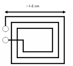
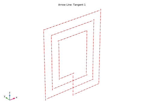
Use the Select Box tool to select the transponder antenna. Verify that the selected edges are 15-23, 29-34, and 38-40.
Reader 1
1
In the Definitions toolbar, click  Explicit.
2
In the Settings window for Explicit, type Reader 1 in the Label text field.
3
Locate the Input Entities section. From the Geometric entity level list, choose Edge.
4
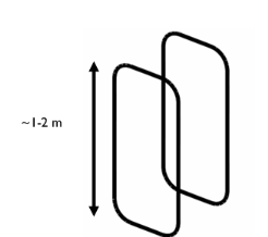
Select all the edges of the reader coil behind the transponder. Verify that you have selected edges 8-10, 13, 14, 43, 44, and 46 only.
Reader 2
1
In the Definitions toolbar, click  Explicit.
2
In the Settings window for Explicit, type Reader 2 in the Label text field.
3
Locate the Input Entities section. From the Geometric entity level list, choose Edge.
4
Select all the edges of the reader in front of the transponder. Verify that you have selected edges 5-7, 11, 12, 41, 42, and 45.
Materials
Add Air as the material for the domain. The coils and the transponder are modeled as ideal edges so no material properties are needed.
Add Material
1
In the Home toolbar, click  Add Material to open the Add Material window.
2
Go to the Add Material window.
3
4
Click Add to Component in the window toolbar.
5
In the Home toolbar, click  Add Material to close the Add Material window.
Materials
Air (mat1)
. The material is applied automatically to all domains.
Magnetic Fields (mf)
Add two Edge Current features to model the coils as ideal line currents. When applying the features on edges, the reference direction for the current flow is indicated by arrows on the edge selection in the Graphics window. A negative value means that the edge current will flow in the direction opposite to the arrow.
Edge Current 1
1
In the Model Builder window, under Component 1 (comp1) right-click Magnetic Fields (mf) and choose Edges>Edge Current.
2
In the Settings window for Edge Current, locate the Edge Selection section.
3
From the Selection list, choose Reader 1.
4
Locate the Edge Current section. In the I0 text field, type 1.
Edge Current 2
1
In the Physics toolbar, click  Edges and choose Edge Current.
2
In the Settings window for Edge Current, locate the Edge Selection section.
3
From the Selection list, choose Reader 2.
4
Locate the Edge Current section. In the I0 text field, type -1.
The default boundary condition for the faces that constitute the sphere is Magnetic Insulation. This allows for surface currents to run across the sphere in such a way as to make the tangential component of the magnetic vector potential equal to zero. This is a good approximation in place of an infinite domain. It approximates that the tangential component of the vector potential approaches zero as the distance from the coils approaches infinity. Thus there is no need to change the boundary settings.
Mesh 1
Size
1
In the Model Builder window, under Component 1 (comp1) right-click Mesh 1 and choose Edit Physics-Induced Sequence.
2
In the Settings window for Size, locate the Element Size section.
3
From the Predefined list, choose Coarser.
4
Click to expand the Element Size Parameters section. In the Minimum element size text field, type 0.0025.
5
Click  Build All.
Study 1
In the Home toolbar, click  Compute.
Results
Magnetic Flux Density Norm (mf)
In the Magnetic Flux Density Norm (mf) toolbar, click  Plot.
Streamline Multislice 1
The default plot shows the magnetic flux density norm in three cross sections. Follow the instructions to get a more informative plot of the fields in the air domain surrounding the coils.
1
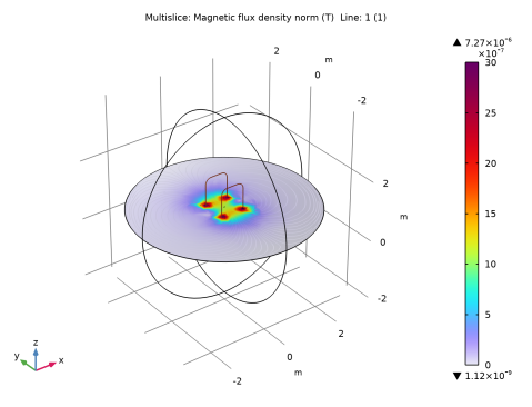
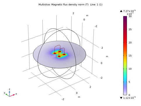
In the Model Builder window, expand the Magnetic Flux Density Norm (mf) node, then click Streamline Multislice 1.
2
In the Settings window for Streamline Multislice, locate the Multiplane Data section.
3
Find the x-planes subsection. From the Entry method list, choose Number of planes.
4
In the Planes text field, type 0.
5
Find the y-planes subsection. From the Entry method list, choose Number of planes.
6
In the Planes text field, type 0.
Multislice 1
1
In the Model Builder window, click Multislice 1.
2
In the Settings window for Multislice, locate the Multiplane Data section.
3
Find the x-planes subsection. From the Entry method list, choose Number of planes.
4
In the Planes text field, type 0.
5
Find the y-planes subsection. From the Entry method list, choose Number of planes.
6
In the Planes text field, type 0.
7
In the Magnetic Flux Density Norm (mf) toolbar, click  Plot.
The plot is dominated by the singular flux density where the reader antennas intersect the slice. One way to suppress the singularities in the plot, is by modifying the color range.
8
Click to expand the Range section. Select the Manual color range check box.
9
In the Minimum text field, type 0.
10
In the Maximum text field, type 3E-6.
11
In the Magnetic Flux Density Norm (mf) toolbar, click  Plot.
Next, add a line plot to reproduce Figure 1.
Line 1
1
In the Model Builder window, right-click Magnetic Flux Density Norm (mf) and choose Line.
2
In the Settings window for Line, locate the Expression section.
3
In the Expression text field, type 1.
4
Locate the Coloring and Style section. From the Line type list, choose Tube.
5
In the Tube radius expression text field, type 1[cm].
6
Select the Radius scale factor check box.
Selection 1
1
Right-click Line 1 and choose Selection.
2
In the Settings window for Selection, locate the Selection section.
3
Click  Paste Selection.
4
In the Paste Selection dialog box, type 5 6 7 8 9 10 11 12 13 14 41 42 43 44 45 46 in the Selection text field.
5
Material Appearance 1
1
In the Model Builder window, right-click Line 1 and choose Material Appearance.
2
In the Settings window for Material Appearance, locate the Appearance section.
3
From the Appearance list, choose Custom.
4
From the Material type list, choose Copper.
5
In the Magnetic Flux Density Norm (mf) toolbar, click  Plot.
As a final step, evaluate the mutual inductance by integrating the magnetic vector potential along the transponder coil; first, analyze the verification of the intended transponder coil direction, then perform the integral.
Transponder Currents Direction
1
In the Home toolbar, click  Add Plot Group and choose 3D Plot Group.
2
In the Settings window for 3D Plot Group, locate the Plot Settings section.
3
Clear the Plot dataset edges check box.
4
In the Label text field, type Transponder Currents Direction.
Arrow Line 1
1
Right-click Transponder Currents Direction and choose Arrow Line.
2
In the Settings window for Arrow Line, locate the Expression section.
3
In the x-component text field, type t1x.
4
In the y-component text field, type t1y.
5
In the z-component text field, type t1z.
Selection 1
1
Right-click Arrow Line 1 and choose Selection.
2
In the Settings window for Selection, locate the Selection section.
3
From the Selection list, choose Transponder.
4
In the Transponder Currents Direction toolbar, click  Plot.
5
Click the  Zoom Extents button in the Graphics toolbar.
6
Click the  Show Grid button in the Graphics toolbar.
Line Integration 1
1
In the Results toolbar, click  More Derived Values and choose Integration>Line Integration.
2
In the Settings window for Line Integration, locate the Selection section.
3
From the Selection list, choose Transponder.
4
Locate the Expressions section. In the table, enter the following settings:
5
Click  Evaluate.
Table
1
Go to the Table window.
The result should be close to 0.99 nH.