Response Spectrum Analysis Theory
Response spectrum analysis is used for computing an approximation of the structural response to transient, nondeterministic events, such as earthquakes or shocks. The idea is that the event is characterized by the peak response that it would give a single degree of freedom (SDOF) oscillator having a certain natural frequency and damping ratio. This response value is provided as a function of the natural frequency of the oscillator. The actual load history of the event is not known explicitly.
This theory section contains:
-
-
-
-
-
-
-
-
-
-
-
-
-
-
-
-
-
-
-
-
Single Degree of Freedom System
Response spectrum analysis is based on the response of a set of single degree of freedom (SDOF) systems.
Consider a mass-spring-damper system, attached to a moving base. The base movement is b(t).
The equation of motion for the mass can, if there are no external loads, be written as
Dividing by the mass, and using customary notation,
Here, the undamped natural (angular) frequency is
and the damping ratio is
It can be seen that the support movement acts as a forcing term, and that the solution depends only on two parameters ω0 and ζ, and not on the individual values of m, c, and k.
Instead of using the absolute displacement as DOF, one can use the relative displacement between the mass and the base,
The equation of motion can then be stated as
(3-143)
In practice, such approach means a frame transformation, where the support movement appears as a gravity-like load.
Definition of a Response Spectrum
For given values of ω0, ζ, and b(t), it is a trivial task to solve Equation 3-143 for the whole duration of the event plus some extra time to allow for the response to reach a possible maximum. The acceleration, velocity, and displacement response spectra are defined as
These are absolute spectra. One can do a similar definition of the relative spectra by using instead the relative displacement ur. It is clear from the definition that there is not a one-to-one relation between the response spectrum and the base acceleration history. The response spectrum gives information about the peak value, but not about when it occurs.
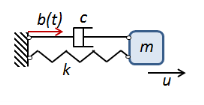
The velocity and acceleration response spectra often are approximated by
Such spectra are called the pseudovelocity spectrum and the pseudoacceleration spectrum, respectively. The expressions contain an assumption about harmonic motion, so that the response is dominated by the homogeneous solution to the equation of motion.
Solution Using Response Spectrum
Assume that one has a structure discretized by FEM, so that the equations of motion on matrix form are
(3-144)
Now, let the structure be connected to a common “ground” at a number of points. These points then have a base motion given by
Let b(t) be a vector that has the same size as the displacement vector u (the total number of DOF), but it contains only three different values: bx(t) in all x-translation DOFs, by(t) in all y-translation DOF, and bz(t) in all z-translation DOF. The relative displacement is now ur = u − b. With no external load, Equation 3-144 can be written as
or
Then, the fact that a rigid body motion does not give any elastic or viscous forces has been used, so that
By solving the undamped eigenvalue problem
with the grounded nodes being fixed, a set of eigenmodes that can represent the relative displacements is obtained. Since the mode displacements are zero at the support points, it is however clear that the modes cannot represent the absolute displacements, for which the support points are moving.
By standard operations for mode superposition (and assuming mass matrix normalization and a diagonalizable damping matrix) the decoupled modal equations are
(3-145)
The equation is similar to the standard SDOF system in Equation 3-143.
In Equation 3-145, qj is the modal coordinate for mode j, so that the relative displacement can be written as a superposition of the eigenmodes .
The support motion can be written as
(3-146)
The notation 1x mean a vector that has the value 1 in all DOF representing x-translation, and the value 0 in all other DOF. Inserting Equation 3-146 in Equation 3-145 gives
The multipliers Γkj are the modal participation factors defined as
Thus, the maximum amplitude of mode j, when loaded by a base motion described by a response spectrum in direction k, is
or, using the pseudoacceleration spectrum
In practice, several modes will have natural frequencies in the frequency range covered by the Design Response Spectrum. This means that a superposition is needed. There are several rules for how this superposition can be done, as will be described in detail below.
Mode Summation
The summation rules are nonlinear. Thus, all result quantities must be summed based on its own modal response. For example, stress components are computed using the modal stresses and cannot be recovered from the response spectrum superposition of displacements.
The general approach is to consider the excitation in three directions, I, (I = 1,2,3) separately. First all modal responses are summed for each direction, and then the results for the three directions are summed. Some methods, however, do both combinations in one sweep.
In a high frequency mode, the mass of the SDOF oscillator will mainly be translated in phase with the support. Such modes constitute the rigid modes. Their responses are synchronous with each other (and with the base motion). This means that for rigid modes, a pure summation should be used, since they are fully correlated.
Modes with a significant dynamic response constitute the periodic modes. The maximum value for such modes will be more or less randomly distributed in time since their periods differ. For this reason, the periodic part of the response requires more sophisticated summation techniques. A plain summation of the maximum values will in general significantly overestimate the true response.
Modes which are in a transition region will partially contribute to the periodic modes, and partially to the rigid ones.
In addition, it is sometimes necessary to add some static load cases, containing a missing mass correction. The reason is that when only a limited set of eigenmodes is used in the superposition, those modes do not represent the total mass of the structure.
In the following, RI denotes any result quantity caused by excitation in direction I. RI can be for example be displacement, velocity, acceleration, strain component, stress component, equivalent stress, or a beam section force. The periodic part of RI is denoted RpI, and the rigid part is denoted RrI. Similarly, RpI,j and RrI,j denote the results from an individual eigenmode j.
Not all analyses require a separation into periodic and rigid modes. In such case, all modes are treated as periodic.
Partitioning into Periodic and Rigid Modes
Figure 3-31: A schematic tripartite plot of a design response spectrum. Both axes have logarithmic scales.
There are two different methods in use, by which the partitioning can be done. In either case, for mode j,
This definition has the property that
The difference between the two methods lies in how the coefficients αj are determined. For low frequencies, it should approach the value 0 (fully periodic modes). And for high frequencies, the value is 1 (fully correlated rigid modes).
The Gupta Method
In the Gupta method, αj is a linear function of the logarithm of the natural frequency.
where f1 and f2 are two key frequencies. Thus, for eigenfrequencies below f1, the modes are considered as purely periodic, and above 
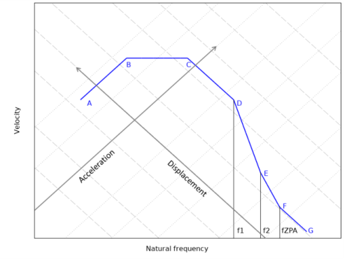
f2 as purely rigid. In the original Gupta method, the lower key frequency is given by
where Sa,max and Sv,max are the maximum values of the acceleration and velocity spectra, respectively. In the idealized spectrum shown in Figure 3-31, this exactly matches the point D.
The second key frequency should be chosen so that the modes above this frequency behave as rigid modes. The frequency can be taken as the one where response spectra for different damping ratios converge to each other.
The Lindley–Yow Method
In the Lindley–Yow method, the coefficient αj depends directly on the response spectrum values, and not only on the frequency. As a consequence, it is possible that a certain mode can be considered as having a different degree of rigidness for different excitation directions
The so-called zero period acceleration (ZPA) is the maximum ground acceleration during the event
This is the high frequency asymptotic value of the absolute acceleration (or pseudoacceleration). It also corresponds to the F-G part of the spectrum in Figure 3-31.
Thus,
The value of αj must be in the range from 0 to 1, and it must increase with frequency. For this reason, NRC RG 1.92 requires that αj must be set to zero for any eigenmodes below point C in Figure 3-31. For a general spectrum, this is implemented as a strict requirement that αj has a monotonous decrease with decreasing frequency from fZPA. As soon as an increase in αj is found, the value is set to zero for all lower frequencies.
Combining Periodic and Rigid Modes
Once the periodic and rigid responses have been summed up separately, they are combined as
Summing the Periodic Modes
All summation rules for periodic modes except Absolute Value Sum can be summarized by the following expression:
Here, RpI is the total periodic response of some result quantity R with respect to excitation in direction I (I=1,2,3). RpI,j is the result from an individual eigenmode j, and N modes are used in the summation. The interaction between the modes is determined by the coefficient Cij (). The different evaluation methods vary only in the definition of Cij.
Since Cij is symmetric and Cij = 1 when i = j, it is more efficient to use the expression
The result quantity R is computed using the ordinary definitions of how a variable is obtained from the DOF fields. This can be expressed as R = g(u). The operator g is however applied to the mode shape, multiplied by a scalar (spectrum value times participation factor)
Next, the different evaluation methods are presented.
SRSS Method
In the SRSS method, it is assumed that the modes are statistically independent, so that
Grouping Method
The modes are grouped according to the following rule:
1
Start a new group m, by inserting the lowest, not yet grouped eigenmode k.
2
3
4
When 3 is not fulfilled any longer, go back to 1.
There are now a number of groups (where some could contain just a single eigenmode), and the coupling coefficient are defined as
The use of the sign function indicates that the term is always added with a positive sign, that is a cross term can never decrease the total sum. There is also an option to allow signed contributions, so that
Ten Percent Method
The ten percent method is similar to the grouping method, and has the following definition:
As can be seen, the ten percent method will always give a higher value than the grouping method, since all pairs that are inside a group will also fulfill the criterion for including the cross term. As in the previous method, there is also an option to use summation with signs, in which case
Double Sum Method
In the double sum method, the correlation between two modes depends on three factors:
Note that there exist two distinct versions of this method. In NRC Regulatory Guide 1.92 revision 1, the mode correlation coefficient is given by
whereas in revision 2 and later version of the same Regulatory Guide the expression is
The latter expression should be considered as more correct and in line with the original theory.
The modified frequency, , is defined as
where ζi is the modal damping. In the implementation in COMSOL Multiphysics, all modes are assumed to have the same damping.
The modified damping, , is defined as
where td is a separate input, called the time of duration. The value of differs between modes, even though the damping is constant.
Der Kiureghian Correlation Coefficient (CQC)
This method, which is often called complete quadratic combination (CQC), is similar to the previous double sum method. The general expression contains modal damping values. Given that a single damping value is used here, the mode correlation expression can be simplified to
(3-147)
Absolute Value Sum
This is the most conservative method, where the peak responses for all modes are summed
This would happen only if all modes reached their peaks simultaneously.
Summing the Rigid Modes
There are two possible combination methods for summing the rigid modes. The method is chosen implicitly, depending on other settings.
Rigid Mode Combination Method A
This is the more common method. The rigid modes are summed algebraically as
where Rmm,I is the term for the missing mass correction, if used.
Rigid Mode Combination Method B
This method is only used when the Lindley–Yow method is used together with the Static ZPA missing mass correction. In this case, the whole rigid mode contribution comes from the static load case, so that
Missing Mass Correction
In general, a mode superposition using a limited number of modes will miss some mass. With the assumption that the higher order modes do not have any dynamic amplification, it is possible to device a correction by solving some extra static load cases, containing the acceleration excitation acting on the 'lost' mass. So-called static correction can be used for mode superposition in general. For the case of response spectrum analysis, the expressions are somewhat simplified.
In terms of the assembled finite element equations, the static correction load fc can be written as
Here, f is the original load vector, M is the mass matrix, and rk are the modal loads, given by the projection of the load vector on the eigenmodes ,
In the base excitation context when response spectrum analysis is used,
so the modal load is
Thus, the missing mass load is
For the rigid body modes, the maximum ground acceleration during the event is equal to the ZPA. The static load is thus
(3-148)
The extra displacement correcting for the missing mass is then given by the standard stationary problem
To actually compute the load in Equation 3-148, the participation factors from a corresponding eigenfrequency study step are needed. The structure of the load is similar to that of a gravity load, but with the acceleration of gravity replaced by the space-dependent field
(3-149)
The load is implemented by using Gravity nodes in the Structural Mechanics interface. The sum of the products between participation factors and mode shapes is performed in a Combined Solutions study step.
The Static ZPA Method
In this method, there is no need to deduce the actual missing mass. It can only be used together with the Lindley–Yow method. According to the Lindley–Yow method, all rigid modes have acceleration SZPA. This acceleration is given to the whole structure. The static load cases are thus just pure gravity loads, but scaled by SZPA instead of the acceleration of gravity.
Summation Over Spatial Directions
The three orthogonal directions in which the design response spectrum is applied cannot, in general, be chosen arbitrarily. The structure may be more susceptible to excitation in a certain direction.
For earthquakes, it is usually assumed that the excitations in the three orthogonal directions are statistically independent. In most cases, there is no reason to assume that the excitations in the two horizontal directions have different spectral properties. Thus, a single design response spectrum is used in the two horizontal directions, and a different one is used in the third vertical (Z) direction.
Often, it is reasonable to assume that the excitations in the two horizontal directions have different amplitudes, even though they share the same spectral properties. The spectrum in the local Y direction is then a scaled version of the spectrum in the local X direction.
The X direction is not a property of the geographical location, but should be chosen as the one giving the worst case for a certain structure. The loading direction which causes the highest response may however not be the same for different result quantities, or for different locations in the structure. For some structures, there is an obvious “weak” direction which can then be chosen as X direction. More often, this is not the case. There are then three possible approaches:
Use the same spectrum in both horizontal directions, that is γ = 1. This will be a conservative approach.
Run a number of separate analyses where the X direction is rotated to different orientations. If 15 degrees can be considered as a small enough rotation increment, then seven analyses are needed.
SRSS Method
In the SRSS (square root of sum of squares) method, the total resultant is computed as
This expression contains an assumption of a statistical independence between the peak responses in three directions.
100-40-40 Method (Percent Method)
In this method, the contribution from the worst direction is taken at full value, whereas the two other contributions are reduced. There are two variants in commonly in use, the 40% (100-40-40) method and the 30% (100-30-30) method. The interpretation is clear: at the time when the peak values is reached in the worst direction, the values in the other direction are not higher than 40% (or 30%) of their individual peak values.
Let the response for the three directions be reordered so that
The total response for the 40% method is then computed as
In some formulations of this rule, the renumbering is not done, and the expression is written instead as
In practice, the same result is obtained as long as signs are properly taken into account when summing the results for multiple responses.
The 40% method is mostly slightly conservative when compared to the SRSS summation. The 30% method is significantly less conservative, and it will often give lower predictions than the SRSS method.
The percent methods are not spatially isotropic. For a symmetric structure, members which for symmetry reason should have the same level of loading will not experience that. The orientation of the reference axes for the acceleration orientation will matter.
CQC3 Method
The CQC3 method extends the CQC principles also to the spatial combination. In the CQC3 method, the modal and spatial combination are performed simultaneously. It is however only formally applicable if only the periodic modes are taken into account.
As in the standard CQC method, the modal response for each loading direction is summed as
where the Der Kiureghian expression Equation 3-147 for Cij is used.
In addition, a similar expression giving the cross coupling between the responses to the spectra in the two horizontal directions is formed:
It is now conceptually assumed that the response spectra are instead applied in a local coordinate system X'-Y' which is rotated an angle θ with respect to the X-Y orientations. It can then be shown that
Also, if the relation between the two spectra in the horizontal plane is such that
the same ratio γ will apply to the responses. The peak response as function of the rotation angle is obtained by an SRSS type summation
It can be seen that for γ = 1, the standard SRSS expression is retrieved.
The angle θmax giving the maximum response R(θmax) turns out to be independent of γ, and it has the value
There are two roots for θmax, both of which must be checked.
The attractiveness of the CQC3 method is that the same spectrum can be applied to an arbitrary pair of orthogonal axes. The scaling of the secondary spectrum, as well as the orientation of the worst direction, is taken care of by the method.
Extending to Rigid Modes
As mentioned above, the original CQC3 method only deals with the periodic part of the solution, so it is limited to cases dominated by such modes. It is however possible to make an extension taking also the rigid (high frequency) modes.
Studying how the rigid modes enter the problem when using CQC (or any of the similar combination rules) together with SRSS spatial combination gives some insight:
Thus, the rigid responses enter the final results as an extra mode, not coupled to the periodic modes. Define a cross term also for the rigid response
Now, it is possible to have the rigid modes too in a CQC3 context. Another way of expressing this is that the rigid response is treated as mode 1, the summation in the CQC3 rule is extended to 1, and
In the GUI, this extension is selected by checking the Augment with rigid response check box.
SRSS3 Method
The SRSS3 method is a special case of the CQC3 rule, in which the mode correlation is ignored, that is
It retains the property of selecting the worst orientation, through the search for θmax. The extension to rigid modes is the same as for CQC3.