In the continuum damage mechanics formalism, a damage variable represents the amount of deterioration due to crack growth. This damage variable controls the weakening of the material’s stiffness, and it produces a nonlinear relation between stress and strain.

For a linear elastic material, Hooke’s law relates the undamaged stress tensor σun to the elastic strain tensor:

here, is the fourth order elasticity tensor, “:” stands for the double-dot tensor product (or double contraction). The elastic strain εel is the difference between the total strain ε and inelastic strains εinel. There may also be an external stress contribution σex, with contributions from initial, viscoelastic, or other inelastic stresses.

For the scalar damage models, the damaged stress tensor σd is computed from the undamaged stress as

This damaged stress is then used in the weak formulation. There are different ways to compute the scalar damage variable d that controls the material weakening. These are listed in the following sections.

The strain-based formulation for the Scalar damage and the Mazars damage for concrete models is based on the loading function f such as

here, εeq is the equivalent strain, a scalar measure of the elastic strain; and κ is a state variable. The evolution of the state variable κ follows the Kuhn–Tucker loading/unloading conditions

In this formulation, κ is the maximum value of εeq in the load history. The damage variable d is then computed as a function of the state variable κ and other parameters.

Different damage models use different definitions for the equivalent strain εeq. The Rankine, stress damage model defines the equivalent strain from the largest undamaged principal stress σp1 as

here, the symbol “<>” represents the Macaulay brackets, and E is Young’s modulus. The Macaulay brackets are used since in this formulation only tensile (positive) stresses cause damage.

Similarly, the Rankine, strain damage model defines the equivalent strain from the largest principal elastic strain εelp1 as

The Smooth Rankine, stress damage model defines the equivalent strain from the three undamaged principal stresses

In the same way, the Smooth Rankine, strain damage model defines the equivalent strain from the three elastic principal strains

By default, only the principal stresses in tension contribute to the damage evolution, for both the Rankine and the Smooth Rankine damage models; but it is also possible to include damage in compression by incorporating the compressive stresses in the computation of the damaged stress tensor σd.

The Euclidean Norm of the elastic strain tensor can also be used as a measure for the equivalent strain

For the Mazars damage for concrete model, it is also possible to select from Mazars or Modified Mazars equivalent strain. Mazars equivalent strain is defined as

In the modified Mazars equivalent strain (Ref. 2 and Ref. 3), a correction factor γ is added to improve the approximation of the failure surface of concrete in multiaxial compression.

It is also possible to apply a User defined expression for defining the equivalent strain as a function of undamaged stress, stress components or strains.

A key component in a scalar damage model is the definition of the damage evolution law. The Linear strain softening law defines the damage variable from

Here, ε0 denotes the onset of damage, computed from the tensile strength σts and Young’s modulus E, so that ε0 = σts/E. The parameter εf is derived from other material parameters such as the tensile strength, the characteristic element size hcb and the fracture energy per unit area Gf, or the fracture energy per unit volume gf.

The Exponential strain softening law defines the damage evolution from

The Polynomial strain softening law defines the damage evolutions from

with εf according to Equation 3-116.

The Multilinear strain softening law defines the damage evolutions from

with εf according to Equation 3-116 and

where λ is an input parameter that defines the shape of the curve.

The Mazars damage for concrete utilizes two different damage evolution laws, one for tensile damage and another for compressive damage. These two damage functions are combined as

here, αt and αc are weight functions depending on the current stress state, and β is the so-called shear exponent which determines the response in shear, that is, the evolution of the combined damage function in states where both damage functions are active.

To define the tensile damage evolution law dt(κ) (Ref. 3), it is possible to use either Linear strain softening, Exponential strain softening, described in Damage Evolution section; or Mazars damage evolution function. A tensile Mazars damage evolution function is obtained by a combination of linear and exponential strain softening

Here, At and Bt are tensile damage evolution parameters, and ε0t is the tensile strain threshold.

The compressive Mazars damage evolution function dc(κ) is obtained by

Here, Ac and Bc are compressive damage evolution parameters, and ε0c is the compressive strain threshold. Both the tensile and compressive damage evolution laws can also be specified by User defined expressions.

The most common application for the damage models is to describe strain localization, due to cracking in quasi-brittle materials. In a damage model without regularization, the deformation during strain softening will always localize in the narrowest possible band, following the principle of least action. This means that large strains will develop in a narrow band of elements (or even Gauss points). As a consequence, the amount of energy dissipated during softening will decrease upon mesh refinement. The results of a damage model without regularization will therefore be mesh dependent and possibly unstable; hence the need for these models to be regularized for the solution to maintain its mesh objectivity.

The simplest regularization method is to modify the stress-strain relation to account for the mesh size. More advanced regularization techniques introduce length scales in the constitutive equation, and additional equations and variables acting as localization limiters. The following sections describe the two methods for damage regularization available in COMSOL Multiphysics.

This simplest regularization technique is based on stress-strain curves (damage evolution laws) that depend on the mesh and element characteristics. The method is often called the Crack Band method (Ref. 4, Ref. 5). The method regularizes the solution from a global viewpoint, which dissipates the correct amount of energy during strain localization. The main difficulty when using the crack band method is to find the correct width of the crack band, hcb; which can depend on the element size and shape, as well as the order of the interpolation and the current stress state (that is, the inclination of the crack with respect to the mesh).

The length scale used in the crack band method is computed by using the volume to area ratio in the mesh elements. By using the element volume v in 3D or the area a in 2D, the crack bandwidth hcb is defined as:

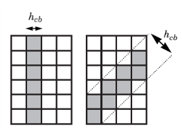
The crack band width hcb is then used to modify the Damage Evolution law in which the damage variable d(κ) is computed. Note that the damage evolution laws (Equation 3-123 and Equation 3-124) are unaffected by the crack band method.

The Implicit Gradient method (Ref. 6) enforces a predefined width of the damage zone through a localization limiter. This is achieved by adding a nonlocal strain variable, the nonlocal equivalent strain εnl, through an additional PDE where the equivalent strain εeq acts as source term. This PDE is solved simultaneously with the displacement field:

Here, the parameter c controls the width of the localization band. This parameter is defined from the internal length scale, lint, and the geometry dimension n (two or three dimension)

If the fracture energy per unit area is used to define the softening behavior, the size of the damage zone is also needed as input. This parameter does not necessarily have the same value as lint.

The strain-based formulation for the damage model (Equation 3-107) is then redefined by the nonlocal equivalent strain εnl instead of the equivalent strain εeq

A rate dependency can be introduced to the damage model by using the Delayed damage viscous regularization method available for time-dependent studies. The method can be used to model a real rate-dependent fracture problem, as well as for stabilizing a rate-independent problem. In both cases, a viscous damage variable dv is introduced. This variable is defined through the following ODE

where τ is the characteristic relaxation time. For the case when the viscous regularization is used to stabilize a rate-independent fracture problem, τ should be significantly smaller than the time step used by the solver in order not to modify the properties of the problem too much. The viscous damage variable dv is then used in Equation 3-106 to define the damaged stress tensor.

The Phase field damage model is closely related to the Strain-based Damage Models, but it is derived from a different starting point. Following a similar derivation as reported in Ref. 7, the model is based on the regularization of a variational formulation of the classical theory by Griffith for brittle fracture; where the geometric crack discontinuity is regularized by a second-order phase field. Including a viscous regularization of the crack phase field φ, the energy functional governing the crack propagation takes the following form:

where d(φ) is the damage function, Ws0 is the elastic strain energy density, η is the viscosity, Gc is the critical energy release rate, and lint is the internal length scale that appears form the regularization of the discrete fracture.

Given the two dependent variables, u and φ, the main contributions to the coupled initial boundary value problem (including inertial terms), are:

where the characteristic time τ and the state variable Hd have been introduced. The state variable Hd is a function of the crack driving force Dd, and it satisfies the Kuhn-Tucker conditions so that:

The momentum balance in Equation 3-130 is included for completeness but is not implemented directly as part of the phase field damage model. However, the equation gives an indication that the damaged stress, as defined by Equation 3-106, is used for the mechanical equilibrium.

The crack driving force, Dd, can be either a function of the elastic strain energy density, or it can also include dissipation processes.

By selecting the Elastic strain energy density, the crack driving force is derived from

where Ws0+ is the tensile part of the undamaged elastic strain energy density. The strain energy threshold Gc0 is an ad hoc variable introduced to establish an elastic threshold before damage occurs. By setting Gc0 equal to zero recovers the model reported in Ref. 7.

By selecting Total strain energy density, additional contributions from dissipative material features, such as creep and viscoelasticity, are added. Select the Calculate energy dissipation check box in the parent material model to compute these variables.

An alternative definition for the crack driving force based on stress measures is suggested in Ref. 8. By selecting the Principal stress criterion, the crack driving force is defined as

where σc is the critical fracture stress, σpi are the undamaged principal stresses, and ξ is a dimensionless parameter which determines the post peak slope.

It is also possible to enter a User defined expression for the crack driving force Dd.

The damage variable d is in the phase field damage model a function of the crack phase field φ. By selecting Power law, the damage evolution function is defined as

where the exponent m is a user input. Often a quadratic function is used so that m = 2. An alternative damage function was suggested in Ref. 9. By selecting Cubic, Borden, the damage evolution function d(φ) reads

where the model parameter s controls the shape of the damage evolution function. The Cubic, Borden option is only available when the crack driving force is defined through the strain energy density.

It is also possible to enter a User defined expression for the damage evolution d as a function of the phase field variable φ.

Typically, phase field damage models use a decomposition of the undamaged strain energy density Ws0 into a tensile and compressive parts. Only the tensile part Ws0+ affects the phase field, and consequently the damage growth and fracture. Several alternative definitions of Ws0+ are available in COMSOL Multiphysics.

The simplest alternative is to set Ws0+ equal to the complete strain energy density Ws0, which means that no split is made into tensile and compressive counterparts. Select No split in the Exclude compressive energy list to achieve this. This option has the advantage that it greatly simplifies the structure of the equations, although that comes at the cost of physical correctness, especially for shear and cyclic loading.

A more accurate method is to use the volumetric-deviatoric split by selecting Volumetric only in the Exclude compressive energy list. Here, only the positive part of the volumetric stress is considered while the entire undamaged deviatoric stress σdev = dev(σun) is included in Ws0+. The definition of Ws0+ then reads

where I1 = trace(σun) is the first invariant of the undamaged stress tensor defined in Equation 3-105 (see Invariants of the Stress Tensor); and εel,vol and εel,dev are the volumetric and deviatoric parts of the elastic strain tensor, respectively (see Invariants of Strain).

Another alternative is to define Ws0+ by performing a spectral decomposition of the stress tensor such that

where σpi are the principal values of the undamaged stress tensor σun, and εel,pi are the principal values of the elastic strain tensor εel (see Principal Strains).

Similarly, a spectral decomposition can be made directly on the elastic strain tensor as suggested in Ref. 7. The tensile part of the elastic strain tensor is then

Both the Spectral decomposition, stress and Spectral decomposition, strain options involve computing the principal values and principal vectors. Such operations are comparatively expensive and typically increase the computational cost of the phase field damage method, however, these are the most correct formulations to use.