Viscoelastic materials have a time-dependent response even if the loading is constant in time. Many polymers and biological tissues exhibit this behavior. Linear viscoelasticity is a commonly used approximation where the stress depends linearly on the strain and its time derivatives (strain rate). Also, linear viscoelasticity deals with the additive decomposition of stresses and strains. It is usually assumed that the viscous part of the deformation is incompressible so that the volumetric deformation is purely elastic.

For isotropic linear elastic materials in the absence of inelastic stresses, Hooke’s law in Equation 3-15 reduces to

where the elastic strain tensor εel = ε − εinel represents the total strain minus initial and inelastic strains, such as thermal strains.

The elastic strain tensor εel can in the same way be decomposed into volumetric and deviatoric components

The total stress in Equation 3-15 is then

In case of geometric nonlinearity, σ represents the second Piola–Kirchhoff stress tensor and εel the elastic Green–Lagrange strain tensor.

For viscoelastic materials, the deviatoric stress σd is not linearly related to the deviatoric strain εd but it also depends on the strain history. It is normally defined by the hereditary integral:

The function Γ(t) is called the relaxation shear modulus function (or just relaxation function) and it can be found by measuring the stress evolution in time when the material is held at a constant strain.

A physical interpretation of this approach, often called the generalized Maxwell model, is shown in Figure 3-1

Hence, G is the stiffness of the main elastic branch, Gm represents the stiffness of the spring in branch m, and τm is the relaxation time constant of the spring-dashpot pair in branch m.

The relaxation times τm are normally measured in the frequency domain, so the viscosity of the dashpot is not a physical quantity but instead it is derived from stiffness and relaxation time measurements. The viscosity of each branch can be expressed in terms of the shear modulus and relaxation time as

The auxiliary strain variable qm is introduced to represent the extension of the corresponding abstract spring, and the auxiliary variables γm = ε − qm represent the extensions in the dashpots.

The shear modulus of the elastic branch G is normally called the long-term shear modulus, or steady-state stiffness, and it is often denoted with the symbol G∞. The instantaneous shear modulus G0 is then defined as the long-term shear modulus plus the sum of the stiffnesses of all the viscoelastic branches

Sometimes, the relaxation function Γ(t) is expressed in terms of the instantaneous stiffness and relative weights, so that the Prony series is given as

and the shear moduli in each branch are defined by the weights wm

The stress per branch can be written either in terms of the strain in the spring, qm, or the strain in the dashpot, γm

The total stress in Hooke’s law (Equation 3-15) is then augmented by the viscoelastic stress σq

The auxiliary variable γm is a symmetric isochoric (volume preserving) strain tensor, which has as many components as the number of strain components of the problem class. Since the stress per branch is written as

the auxiliary variables γm can be computed by solving the ODE

so that Equation 3-27 can equivalently be written as

The viscoelastic strain variables, γm, are treated as additional degrees of freedom (DOFs). The shape functions are chosen to be one order lower than those used for the displacement field, because these variables add to the strains and stresses computed from displacement derivatives. Alternatively, Equation 3-41 can be solved using a Local Time Integration algorithm.

where εel,vol is the elastic volumetric strain, and the auxiliary variables evol,m represent the volumetric deformation per branch. These are computed by solving the ODE

where τm is the relaxation time per branch.

Only branches that have a relaxation time which is of the same order of magnitude as the temporal variation of the loading are important for the viscoelastic response. The cost in terms of memory consumption and computational speed increase significantly if the model contains many branches, particularly in time domain and for eigenfrequency analyses. In these cases many auxiliary equations of the form Equation 3-28 have to be solved for.

When the frequency band of interest is bounded by two cutoff frequencies, flower and fupper, it is possible to prune viscoelastic branches that have relaxation times such as

Branches with short relaxation times τk represent the response of the viscoelastic material to high frequency excitations. When the external loads represent excitations bounded by an upper frequency fupper, it is possible to prune branches with relaxation times that fulfill the relation . These branches are grouped into an equivalent branch, with relaxation time and stiffness such as

Viscoelastic branches with relaxation times τk such that are grouped into an equivalent branch forming the low frequency cutoff. The stiffness and relaxation time for the equivalent branch are computed from

The dissipated energy density rate (SI unit: W/m3) in each dashpot m is

In order to compute the dissipated energy density, the variable is integrated over time. For frequency domain studies, the dissipation of viscous forces averaged over a time period 2π/ω is computed from the shear loss modulus G'' as

The Maxwell model is a simplification of the generalized Maxwell model with only one spring-dashpot branch:

The generalized Kelvin–Voigt model is used to simulate the viscoelastic deformation in a wide range of materials such as concrete, biological tissues and glassy polymers.

Just as for the generalized Maxwell model, the deviatoric strain εd is not linearly related to the deviatoric stress σd, but it also depends on the strain history. It is normally defined by the hereditary integral:

The function ψ(t) is called the compliance function (also called creep compliance or creep function) and it can be found by measuring the strain evolution in time when the material is held at a constant stress.

A physical interpretation of this rheological model consists of an elastic branch plus a number of Kelvin–Voigt elements arranged in series, this approach is shown in Figure 3-3.

Here, G is the stiffness of the main elastic branch, Gm represents the stiffness of the spring in element m, and τm is the relaxation time constant of the spring-dashpot pair in branch m. The compliance J in the pure elastic branch is related to the shear modulus by

The relaxations time τm is normally measured in the frequency domain, so the viscosity of the dashpot is not a physical quantity but instead it is derived from stiffness and relaxation time measurements. The viscosity in each branch can be expressed in terms of the stiffness or compliance modulus and relaxation time as

The auxiliary strain variables γm are introduced to represent the extension of the corresponding Kelvin–Voigt element. Since the elements are arranged in series, the total viscoelastic strain is given as the sum of the auxiliary strains

The deviatoric stress σd in the pure elastic branch is the same as in all the Kelvin–Voigt elements

The auxiliary strain variables γm represent a symmetric isochoric (volume preserving) strain tensor, which has as many components as the number of strain components of the problem class.

The stress in each element m is given by the sum of the stresses in the spring and dashpot arranged in parallel

Here, γm is the strain in the element m, and ηm = τmGm is the viscosity. The auxiliary variables γm are computed by solving the ODE

The compliance of the elastic branch, J = 1/G, is normally called the instantaneous compliance, and it is often denoted with the symbol J0. This gives the equivalent stiffness when the material is loaded by an abrupt load much faster than the shortest relaxation time of any branch.

The long-term compliance J∞ is defined as the instantaneous compliance plus the sum of the compliances of the viscoelastic branches

The long-term shear modulus then reads G∞ = 1/J∞.

Sometimes, the compliance function ψ(t) is expressed in terms of the instantaneous compliance J and relative weights wm, so that the Prony series reads

The dissipated energy density rate (SI unit: W/m3) in each branch m is given by the dissipation in the dashpot

In order to compute the dissipated energy density, the variable is integrated over time. For frequency domain studies, the dissipation of viscous forces averaged over a time period 2π/ω is computed from the shear loss modulus G'' as

The Kelvin–Voigt viscoelastic model is represented by a spring connected in parallel with a dashpot:

so there is no need to add the extra DOFs to compute the auxiliary strain tensor γ.

The relaxation time relates the viscosity and shear modulus by η = τG. The equivalent shear modulus is used in case of an anisotropic linear elastic material.

The standard linear solid model, also called SLS model, Zener model, or three-parameter model, is a simplification of the generalized Maxwell model with only one spring-dashpot branch:

where the relaxation time is related to the stiffness and relaxation time as η1 = τ1G1.

The auxiliary strain tensor γ1 is computed by solving by the ODE

The long-term shear modulus G∞ = G is given in the parent Linear Elastic Material, and the instantaneous stiffness is given by G0 = G+G1.

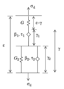
The Burgers model consists of a Maxwell (spring-dashpot) branch in series with a Kelvin–Voigt branch. The rheological representation of this material model is shown in Figure 3-6:

where the shear modulus G is taken from the parent Linear Elastic material.

Combining these equations, it is possible to recover a second-order ODE for the strain tensor γ:

Note that the Burgers material has two relaxation times related to the stiffness and viscosity in the springs and dashpots. The relaxation times τ1 and τ2 are related to the stiffness and viscosities as τ1 = η1/G and τ2 = η2/G2.

The instantaneous stiffness G0 = G is given in the parent Linear Elastic Material.

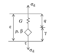
Typically, the rheology of viscoelasticity models consists of springs and dashpots arranged in series and in parallel. Using the framework of fractional calculus, the constitutive equations of linear viscoelasticity can be generalized with a new type of element, named spring-pot (Ref. 38). In some cases, viscoelasticity models with fractional derivatives have shown to better match experimental data.

The basic stress-strain relation of the spring-pot element is given by a proportionality factor p and a fractional time derivative of order β

The fractional order β takes a value between 0 < β < 1. For β = 0, the parameter p plays the role of a stiffness in a spring, and for β = 1 the parameter plays the role of the viscosity in a dashpot. The SI unit for such material parameter would be Pa·sβ.

For a standard spring-dashpot branch, the relaxation time is given by the ratio of viscosity and stiffness, τ = η/G. Equivalently, the relaxation time τ for a branch with a spring and a spring-pot element in series is derived from

Thus, p = τβ/G, and the stress-strain relationship in the spring-spring-pot system reads

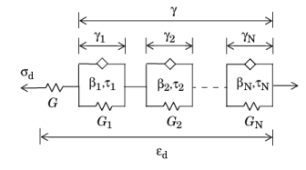
For The Generalized Maxwell Model with fractional derivatives, all dashpots are replaced with spring-pot elements. The rheological representation of this material model is shown in Figure 3-9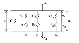

where Gm, τm and βm are the shear modulus, relaxation time and fractional order of branch m, respectively. Storage and loss moduli are defined as the real and imaginary part of the complex shear modulus.

The relaxation time τ for a spring and a spring-pot element in parallel is derived from

so p = τβ/G, and the stress-strain relationship in the Kelvin–Voigt element reads

The complex-valued compliance of the Kelvin–Voigt element with fractional time derivative reads

For The Generalized Kelvin–Voigt Model with fractional derivatives, all dashpots are replaced with spring-pot elements.

The rheological representation of this material model is shown in Figure 3-11.

where Gm, τm and βm are the shear modulus, relaxation time and fractional order of element m, respectively. Storage and loss moduli are defined as the real and imaginary part of the complex shear modulus

In the rheological representation of the Standard Linear Solid Model with fractional derivatives, the dashpot is replaced with a spring-pot element.

here, γ1 is the strain in the spring-pot element. In frequency domain this equation translates to

Using the relaxation time τ = (p/G1)1/β, this reads

where Gq = G1(jωτ)β/(1+(jωτ)β) is the complex shear modulus of the spring-pot branch.

The storage and loss moduli are defined as the real and imaginary parts of the shear modulus GSLS, respectively

In the rheological representation of The Burgers Model with fractional derivatives, the dashpots are replaced with a spring-pot elements. The rheological representation of this material model is shown in Figure 3-13:

here, γ1 is the strain in the spring-pot element. In frequency domain, and using the relaxation times τ1 = (p1/G)1/β1, this equation translates to

here, γ2 is the strain in the second spring-pot element. In frequency domain, and using the relaxation time τ2 = (p2/G2)1/β2, this equation reads

The storage and loss moduli are defined as the real and imaginary parts of the shear modulus GB = 1/JB, respectively

With the user-defined viscoelastic material model it is possible to directly enter complex-valued expressions for the bulk and shear moduli or compliances, or for the loss factor. The bulk and shear moduli or compliances are entered in terms of storage and loss moduli or compliances, respectively. The expressions can be entered as functions taken directly from interpolated data, or can be analytical expressions of the frequency variable ω.

where D is the constitutive matrix computed from the material data, and Dc is the complex constitutive matrix used to compute the viscoelastic stresses.

For many polymers, the viscoelastic properties have a strong dependence on the temperature. A common assumption is that the material is thermorheologically simple (TRS). In a material of this class, a change in the temperature can be transformed directly into a change in the time scale. The reduced time is defined as

where αT(T) is a temperature-dependent shift function.

Think of the shift function αT(T) as a multiplier to the viscosity in the dashpot in the Generalized Maxwell model. This multiplier shifts the relaxation time, so Equation 3-28 for a TRS material is modified to

where a base-10 logarithm is used. This shift is only valid over a certain temperature range, typically around the glass transition temperature.

The first step to compute the shift function αT(T) consists of building a master curve based on experimental data. To do this, the curves of the viscoelastic properties (shear modulus, Young’s modulus, and so forth) versus time or frequency are measured at a reference temperature Tref. Then, the same properties are measured at different temperatures.

The shift value of each curve, with respect to the master curve obtained at the temperature Tref, defines the shift factor αT(T). The constants C1 and C2 are material dependent and are calculated after plotting log(αT) versus T − Tref.

Since the master curve is measured at an arbitrary reference temperature Tref, the shift factor αT(T) can be derived with respect to any temperature, and it is commonly taken as the shift with respect to the glass transition temperature. The values C1 = 17.4 and C2 = 51.6 K are reasonable approximations for many polymers at this reference temperature.

Below the Vicat softening temperature, the shift factor in polymers is normally assumed to follow an Arrhenius law. In this case, the shift factor is given by the equation

here, a base-e logarithm is used, Q is the activation energy (SI unit: J/mol), and R is the universal gas constant.

here, a base-e logarithm is used, Q is the activation energy (SI unit: J/mol), R is the universal gas constant, T is the current temperature, Tref is a reference temperature, χ is a dimensionless activation energy fraction, and Tf is the so-called fictive temperature. The fictive temperature is given as the weighted average of partial fictive temperatures.

Here, wi are the weights and Tfi are the partial fictive temperatures. The partial fictive temperatures are determined from a system of coupled ordinary differential equations (ODEs) which follow Tool’s equation

here, λ0i is a structural relaxation time.

The instantaneous shear modulus G0 is defined as the sum of the stiffness of all the branches

Equation 3-26 and Equation 3-28 are then simplified to

where the shear storage modulus G’ and the shear loss modulus G” are defined for the generalized Maxwell model as

The internal work of viscous forces averaged over a time period 2π/ω is computed as

The direct use of frequency-dependent shear or bulk moduli, as described in Frequency Domain Analysis and Damping, leads to a nonlinear eigenvalue problem. COMSOL Multiphysics solves such nonlinear problems by expanding all nonlinear expressions with quadratic polynomials around a frequency linearization point which you can specify in the Eigenvalue Solver node. The linearized eigenvalue problem then reads

where ωL is the angular frequency at the linearization point. Thus, the solution of the linearized system of equations depends on the choice of the linearization frequency ωL.

Selecting the linearization frequency closer to one of the eigenfrequencies will produce a better result for that particular frequency, but not for all eigenfrequencies in the study. Hence, the eigenfrequencies need to be computed one by one using a certain iterative process that updates the linearization frequency ωL. This iterative procedure is needed when fractional derivatives are used, and also for the User Defined viscoelasticity model.

In order to avoid solving a nonlinear eigenvalue problem for the built-in viscoelasticity models, the same procedure as for time-dependent analysis is used, that is, each viscoelastic branch is represented by additional variables. For instance, for the The Generalized Maxwell Model in a eigenfrequency analysis, Equation 3-28 reads

The viscoelastic strain variables, γm, are treated as additional degrees of freedom (DOFs), and contribute to the damping and stiffness matrices of the coupled system of equations.

For the The Generalized Maxwell Model and the Standard Linear Solid Model it is possible to use a local time integration algorithm for time dependent analysis. By using this algorithm, the degrees-of-freedom related to viscoelasticity are treated as internal state variables, which makes the overall solution more efficient and also leaner in terms of memory usage. The implemented algorithm is based on the method originally suggested in Ref. 21, and it is schematically described in the following.

where γm is the viscoelastic strain in the branch. The exact solution to Equation 3-33 is

By assuming that the strain ε(t) varies linearly within each time increment, the integral in Equation 3-34 is analytically computed, so the viscoelastic strain at increment n+1 reads

All variables in Equation 3-35 evaluated at increment n are stored as internal state variables, and the equation can be applied to each branch of the Generalized Maxwell model. The same implementation is also used for the single branch in the Standard Linear Solid model.