Performing a Response Spectrum Analysis
Introduction
Response spectrum analysis is used to approximately determine the structural response to short nondeterministic events like earthquakes and shocks. The idea is that the event is characterized by the peak response that it would give a single degree of freedom (SDOF) oscillator having a certain natural frequency and damping ratio. The response value is provided as a function of the natural frequency of the oscillator.
If the dynamic structural response is viewed as a mode superposition, each eigenmode within the given frequency range acts as an SDOF oscillator, with a peak amplitude that is known from the spectrum. There is, however, no information about when each mode reaches its peak value. The most conservative assumption is that all modes should be combined using the individual peak values. Using such approach will in most cases result into an extremely conservative design. For this reason, other summation methods have been developed. When performing a response spectrum analysis, you will have access to several such methods.
Setting up a Response Spectrum Analysis
The response spectrum analysis is not a study type. The computations are performed during result evaluation. You enter the methods and parameters in the settings for the Response Spectrum 2D or Response Spectrum 3D datasets. These datasets require the following:
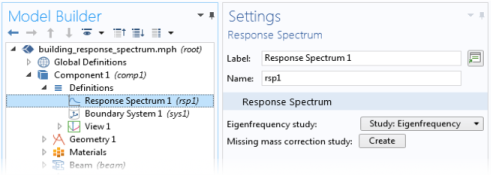
An eigenfrequency solution, where the eigenmodes to be included in the response spectrum analysis have been computed. All computed eigenmodes are used. If you want to filter out a particular set of modes, you can add a Combine Solutions study step after the Eigenfrequency study step. Such a filter can for example be based on the effective modal mass, so that only modes which contribute significantly to the mass are included.
A corresponding set of modal participation factors. To generate them, add a Response Spectrum node under Definitions in the component. If you have computed the eigenfrequency prior to adding the Response Spectrum node, you need to perform an Update Solution.
Adding a Response Spectrum Study
In the Add Study dialog, there is a study type called Response Spectrum. When you select it, two things happen:
A study, containing a single Eigenfrequency study step is created.
A Response Spectrum node is added under Definitions in the first component which contains at least one structural mechanics physics interface. In this node, the Eigenfrequency study list will be initialized to point to the Eigenfrequency study step that was just created.
If you already have computed the eigenfrequencies of a structure, and then want to perform a response spectrum evaluation, there is no need to add a new study. Just add a Response Spectrum node under Definitions->Variable Utilities, and then do an Update Solution to make the new variables available.
Missing Mass Correction
You create a missing mass correction study from the Response Spectrum node by clicking the Missing mass correction study: Create button.
A number of items are then created in the model tree:
A set of load group nodes are created under Global Definitions. There are two load groups for each spatial direction. The load group nodes are placed under a common group named Load Groups for Missing Mass Correction.
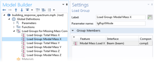
The Parameter name of the load group is reserved, and you should not modify it.
A new study named Study: Missing Mass Load Cases is created. This study contains three or four study steps, depending on the space dimension. First, there is one Combine Solutions study step for each spatial direction. In these steps, a weighted sum of the eigenmodes is computed. The weights are the modal participation factors in each direction. This gives a measure of the mass that the eigenmodes represent.
These study steps must reference the eigenvalue solution, including any subsequent filtering. If you change the study from which the eigenmodes are to be taken, you must also change the choice in the Solution list in all of the Combine Solutions nodes. The final study step in the study is a stationary study step, where each load group is solved separately by adding one load case per load group.
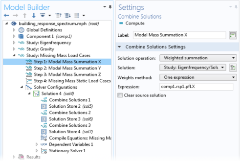
Disable them in this study, by using Modify model configuration for study step in the Physics and Variables section in the settings for the study step. This is the preferred method.
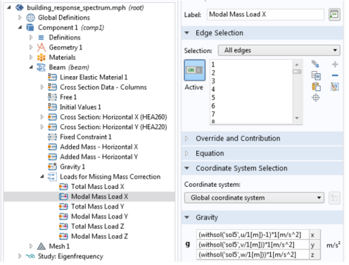
In each structural mechanics physics interface in the component, a set of Gravity nodes are added. There are two such nodes for each spatial direction. Each gravity node is connected to a corresponding load group. Half of the loads are pure gravity loads, used when only together with the Static ZPA method. The other set of loads, which are used in the Missing mass method, are referencing the combined solutions as the depend on the computed eigenmodes. The gravity nodes are placed under a common group, named Loads for Missing Mass Correction.
Settings for the Response Spectrum Datasets
Defining the Spectra
You input the spectra as functions under Global Definitions. Usually, either an interpolation function, or an analytic function, or a piecewise function is used.
There are two common methods to describe the design response spectra: either as function of frequency, or as function of period time. Use the Depends on setting to control this.
The handling of units in the functions are nonstandard:
The unit of the function is not checked. The function will, however, be scaled to model units, so if you, for example, enter the unit mm/s^2 for an acceleration spectrum, the function will (in an SI system) be scaled by 1/1000. You would get the same effect if the entered unit is inconsistent (for example, mm).
The spectra you enter have the following correlation to the spatial directions:
In 3D, you can supply two different horizontal spectra, called primary and secondary horizontal spectrum. Those spectra act in two orthogonal directions, which by default coincide with the global X and Y directions. By giving a nonzero value to Primary axis rotation, you can make the primary spectrum act in an arbitrary direction in the XY-plane.
Some Spatial combination methods in 3D (CQC3 and SRSS3) assume that the two horizontal spectra are equal except for an amplitude scale factor. In such case, you only provide one spectrum together with a Secondary horizontal spectrum scale factor (value between 0 and 1).
Mode Combination
The combination of the eigenmodes is the core of the response spectrum methods. Most commonly the combination is done in two passes: first the response to the excitation in each spatial direction is determined, and then a total response is computed by combining the spatial responses. However, for certain methods the total response is computed in one pass.
First, you select a Spatial combination method. If it is SRSS or Percent method, you also select a Mode combination method.
The mode combination methods require different inputs. In particular, several of them provides a possibility to choose whether the coupling terms between modes are to be considered as always positive, or they may actually reduce the total response. This is controlled by the Use absolute value for coupling terms check box. Its default value differs between the methods, according to what is expected to be the most common choice.
Periodic Modes and Rigid Modes
For frequencies higher than the highest frequency content of the excitation, the SDOF system will respond as a rigid body. Some of the response spectrum evaluation methods take this into account. The effect is that high-frequency (“rigid”) modes are assumed to have a higher degree of correlation than low-frequency (“periodic”) modes. To take this effect into account, you can select Rigid modes to be the Gupta method or the Lindley-Yow method.
Missing Mass Correction
In general, only a small fraction of the total number of eigenmodes are used in the superposition. Therefore, some fraction of the total mass of the structure is not accounted for. The ignored modes usually have high natural frequencies. Such modes will not have a significant dynamic amplification. The mass in the corresponding SDOF system will just follow the movement of the foundation. This means that if the distribution of the missing mass is known, then it can be treated as an extra stationary mass force, where the peak acceleration during the event replaces the acceleration of gravity.
You can use two different methods for missing mass correction:
In the Missing mass method, the difference between the true mass distribution and the mass represented by the used eigenmodes will act as extra static load. Typically, most of the missing mass is located close to support points, where the modal amplitudes are low. This method can be used together with either the Gupta method or the Lindley-Yow method.
In the Static ZPA method, the total inertial force is used as static load. At the same time, only the periodic part of the response is used in the mode summation. This method can only be used together with the Lindley-Yow method because it is only compatible with the assumptions about how the rigid modes are scaled.
Result Interpretation
All results from a response spectrum analysis are positive; the evaluation methods contain absolute values or RMS-like operations. This has important implications for the interpretation of the results:
An underlying implicit assumption for response spectrum analysis is that it is performed in a frame of reference that follows the foundations of the structure. Thus, all displacements, velocities, and accelerations are relative to the foundation, which in itself is accelerating. Thus, it is difficult to evaluate the absolute acceleration. The conservative way of doing so is to add the peak acceleration of the underlying event to the computed acceleration. This will usually be rather conservative since the peak of the excitation seldom coincides in time with the peak of the response.
For displacements, the relative displacements between two objects within the same moving frame is usually a more important result than the absolute displacement, so it does seldom matter whether a constant value is added to all points or not.
The Response Spectrum node is described in the COMSOL Multiphysics Reference Manual.
Combine Solutions and Updating a Solution in the COMSOL Multiphysics Reference Manual.
Earthquake Analysis of a Building: Application Library path Structural_Mechanics_Module/Dynamics_and_Vibration/building_response_spectrum
Shock Response of a Motherboard: Application Library path Structural_Mechanics_Module/Dynamics_and_Vibration/motherboard_shock_response