Theory Background for the Layered Shell Interface

The Layered Shell interface is based on the layerwise theory of modeling a composite laminate. A layerwise (LW) theory is very similar to the traditional 3D elasticity theory where the degrees of freedom are only the displacement fields defined in the product geometry. The product geometry, or a domain, is defined by the reference geometric surfaces and a virtual extra dimension in the thickness direction.


	The key features of the layerwise theory and a comparison with ESL theory and 3D elasticity theory are described in Laminated Shell Theories in the documentation for the Composite Materials Module.

This section covers the following topics:

•

Physics Interface Selection

•

•

•

•

•

•

Layer Materials, Thicknesses, and Orientations

•

Offset and Local Coordinate System

•

Transform and Scale

•

Fold-Line Connection

•

Layered Shell Continuity

•

Using the Extra Dimension Coordinates

•

Results Evaluation in Layered Shells

Physics Interface Selection

A Layered Shell physics interface is defined using a surface (2D) geometry and an extra dimension (1D) geometry in the through-thickness (or normal) direction. The surface geometry is a physical geometry and supposed to be created in the model whereas the extra dimension geometry is a virtual geometry created by and similar nodes.

The geometric surface (or its lower dimension) selection, together with layer (or interface) selection creates the product geometry for the governing equations and boundary conditions of the Layered Shell interface.

The Layered Shell interface itself exists on a domain level which is a product geometry created using selected geometric surfaces and material layers. The physics features can exist on domain level or its lower dimensions. Based on whether a physics feature exists on a layer or an interface, the physics features can be divided into two categories:

•

Layer features (having boundary, edge, or point selection)

•

Interface features (having boundary, edge, or point selection)

Layer features may or may not allow a layer selection. When a layer selection is not allowed, the layer feature is applied to all layers.

Interface features, may allow only exterior interfaces, interior interfaces, or alternatively all interfaces of a laminate.

•

For a general description of layer selections, see Layer and Interface Selections in the documentation for the Composite Materials Module.

•

For a general description of layered materials, see Layered Materials in the documentation for the Composite Materials Module.

Governing Equations

The dependent variable in the Layered Shell interface is the displacement field. The dependent variable is available in the product geometry.

The governing differential equations, constitutive relations, the definition of deformation, stresses, strains are same as in the 3D elasticity theory as described for the Solid Mechanics interface.


	See Solid Mechanics Theory for more details.

Gradient Definition

In the analysis of deformations in 3D, the deformation gradient F is defined as

An equivalent definition of a deformation gradient in a product geometry of a layered shell can be written as

(6-1)

where

•

is the tangential gradient operator

•

is the extra dimension thickness coordinate (varies between 0 and d)

•

is the positive normal direction

Equation 6-1 is exact for flat laminates. For curved laminates, the deformation gradient expression must account for the surface area of each layer. The deformation gradient in a product geometry of a curved layered shell can be written as

where

•

Xr are the reference surface coordinates

•

is the relative midplane offset

•

is the laminate thickness

In some applications, it is required to model variable thickness layers. This is achieved by scaling the constant thickness of the layer (d_layer) using a thickness scale factor (lsc), which could be a function of surface coordinates. The deformation gradient in a scaled product geometry of a curved layered shell can be written as

where

•

is the scaled extra dimension thickness coordinate (varies between 0 and

)

•

is the scaled laminate thickness

Area Scale Factor

For a curved laminate, the change in surface area of each layer should be accounted for while integrating the energy expressions. The area scale factor for each layer of the laminate can be defined as:

Integrations

All volume integrals over a layered shell element are split into a surface integration and a through-thickness integration. Both integrations are performed numerically. The surface geometry is used for surface integration and the extra dimension geometry is used for the through-thickness integration. It is thus possible to enter data which explicitly depends on the thickness direction.

Unlike a single layer shell, where all material properties are evaluated at the reference surface, different material and fiber orientation can be specified in each layer of the composite laminate. Formally this can be written as:

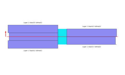
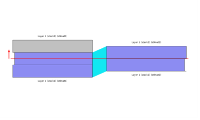
As discussed in the previous section, an area scale factor (ASF) is included for curved laminates since the layers have different surface area. This is independent of whether an offset is used or not, but the offset affects the scale factor.

The layer thickness scale factor (lsc) is also accounted in the integrations when variable thickness layers are present in the model.

Discretization

The Layered Shell interface can use different shape orders for the displacement field in the reference surface and in the through-thickness direction. The shape orders used can be divided into categories:

•

Same shape order in the reference surface and in the extra dimension (Figure 6-3 and Figure 6-4)

•

Different shape orders in the reference surface and in the extra dimension (Figure 6-5)

Based on the above two categories, 9 different elements are available:

•

Linear (8 nodes)

•

Quadratic Lagrange (27 nodes)

•

Quadratic Serendipity (24 nodes)

•

Cubic Lagrange (64 nodes)

•

Cubic Serendipity (48 nodes)

•

Quadratic-Linear Lagrange (18 nodes)

•

Quadratic-Linear Serendipity (16 nodes)

•

Quadratic-Cubic Lagrange (36 nodes)

•

Quadratic-Cubic Serendipity (32 nodes)

Figure 6-3: Element having linear shape order.

Figure 6-4: Elements having quadratic and cubic shape orders.

Figure 6-5: Elements having different shape orders on the reference surface and in the through-thickness direction.

Layer Materials, Thicknesses, and Orientations

A layered shell can have many layers with following different properties in each layer:

•

Material (isotropic, orthotropic, or anisotropic)

•

Thickness

•

Orientation

•

Mesh elements in the through-thickness direction


	For a general description of layered materials, see Layered Materials in the documentation for the Composite Materials Module.

Offset and Local Coordinate System

The position of the reference surface with respect to midplane of the laminate and the local coordinate system in which material properties and results are interpreted can be defined in and similar nodes.


	For a general description of layered materials, see Layered Materials in the documentation for the Composite Materials Module.

Transform and Scale

The transform functionality can be optionally used to simplify the definition of stacking sequence. Various transform options available are symmetric, antisymmetric, and repeated.

The scale functionality can be optionally used to model a variable thickness layer. The scale defined for each layer, which could be a function of reference geometry, is multiplied to the constant layer thickness essentially making it a variable thickness layer.

The transform and scale options can be defined in and similar nodes.


	For a general description of layered materials, see Layered Materials in the documentation for the Composite Materials Module.

Fold-Line Connection

When two or more layered shell surfaces meet at an angle, the displacement field cannot be same on the side faces of all the layered shell surfaces. Thus, a slit condition is needed on the common edges and a connection needs to be established between the displacement field of different layered shell surfaces sharing an edge.

This is automatically handled by the program. The automatic search for these fold lines compares the normals of all the layered shell surfaces sharing an edge. If the angle between the normals is larger than a certain angle (default 3°) it is considered as a fold line.

In order to connect the displacement field of different shell surfaces meeting at a fold line, the following two conditions are needed:

•

The displacement at the reference surface position should be continuous. This can be written as

where

is the displacement vector at the reference surface location in the through-thickness direction.

•

The angle between the shell normals remains constant. This can be written as

where

is the displacement vector in the through-thickness direction relative to the displacement vector at the reference surface location.

Layered Shell Continuity

Different layered materials have their own virtual extra dimension geometry and that is why, by default, two layered materials sharing a common edge in the geometry do not have a continuous displacement field. Thus, when two layered shell surfaces having different layered materials meet side-by-side, a displacement continuity needs to be established in the through-thickness direction on the common edge.

For an example, a layered material having 3 layers shares a common edge with another layered material having 2 layers. For that case, some of the ways you can connect the two layered materials in the through-thickness direction are as follows:

•

Connecting the first and third layer of the left layered material to both the layers of the right layered material. This type of connection is typically used in a ply dropping scenario.

•

Connecting the geometrically common area of both the layered materials in through-thickness direction.

•

Connecting the first two layers of the left layered material to both the layers of the right layered material.


	Note that continuity between different layered materials meeting side by side is correctly established for surfaces having the same normal direction at the common edge. In case the two layered materials have normal orientation in opposite directions, you may want to switch the Connection type from Straight to Twisted in the Connection Settings section of the Continuity node in order to connect points in extra dimension which are geometrically close to each other. Using the continuity condition when the two surfaces meet at an angle may give rise to the stress concentration near the common edge, as well as a locking of the global rotation of the layered shell surfaces.

Using the Extra Dimension Coordinates

Sometimes, you want to write expressions that are functions of the coordinates in the thickness direction of the layered shell. If you write expressions based on the usual coordinates, like X, Y, and Z, such an expression will be evaluated on the reference surface (the meshed boundaries). In addition to this, you can access locations in the through-thickness direction by making explicit or implicit use of the coordinates in the extra dimension.

The extra dimension coordinate has a name like x_llmat1_xdim. The middle part of the coordinate name is derived from the tag of the layered material definition where it is created; in this example a .

You can also access the extra dimension coordinate as wrapped into a physics interface variable, like lshell.xd (varies from 0 to the total laminate thickness d) and lshell.xd_rel (varies from 0 to 1).

Finally, the coordinates in 3D space are available using the physics scoped variables lshell.X, lshell.Y, and lshell.Z. These coordinates vary also in the thickness direction of the layered shell.

You can also write expressions that explicitly contain the number of the layer, available in the variable lshell.num. The number of the bottommost layer is ‘1’.

Results Evaluation in Layered Shells

For visualization and results evaluation, predefined variables include all nonzero stress and strain tensor components, principal stresses and principal strains, in-plane and out-of-plane forces, moments, and von Mises and Tresca equivalent stresses.

Stresses and strains are available in the global coordinate system, laminate coordinate system, as well as in the layer local coordinate system.

Layered Material Slice Plot

It is possible to evaluate the stress and strain tensor components and equivalent stresses in each layer of a laminate using plot.

The through-thickness location can be set to evaluate a quantity in the middle of a layer, at an interface between two layers, top or bottom of a laminate etc. The top, bottom, and the middle of a laminate can be defined as:

•

Bottom of a laminate: −1 (relative) and 0 (physical)

•