Frozen Inclusion

This benchmark example simulates phase change in porous media. The model studies the melting process of an ice inclusion within a porous medium, and it demonstrates how to couple Darcy’s Law and the Heat Transfer in Porous Media interfaces including phase change. It is one of the test cases from the INTERFROST project — a comparison project for coupled thermo-hydraulic systems with respect to climate change in permafrost regions (see Ref. 2).

Model Definition

The model setup is shown in Figure 1. A flow channel 3 meters in length and 1 meter in width contains a squared ice inclusion of 33.3 cm in length, centered at the coordinates x = 1 m and y = 0.5 m.

Figure 1: Model geometry, initial temperature distribution, and boundary conditions.

The initial temperature of the ice inclusion is Tini = −5°C. The temperature in the porous channel is Tinw = +5°C. The fluid flow is driven by a hydraulic head gradient of ΔH = 3% over the length of the channel.

The initial pressure and velocity field are computed from a steady state flow simulation for a uniformly distributed temperature and permeability (as if the ice inclusion was not present). Considering the symmetry of the benchmark test model, only the lower half of the domain is modeled.

The following simplifications have been made in the INTERFROST benchmark and therefore are also assumed in this example: No thermal dispersion is included in the heat transfer equation, and water density and dynamic viscosity are considered constant with respect to the temperature (see Table 1).

Model equations

The Porous Medium feature in Darcy’s Law interface includes an option to define a user-defined storage Sp (SI unit: 1/Pa) which in this case is defined as

(1)

where Sw is the water saturation, εp is the porosity, and β the effective compressibility; which is a combined value of water, ice, and solid matrix compressibility. For simplicity, gravity is neglected. The variable Qm is a mass source which represents the additional liquid water due to the melting of the ice inclusion:

(2)

here ρi and ρw are the ice and liquid water densities. The liquid water saturation Sw depends on the phase change as:

(3)

here, Sw, res it the residual liquid water saturation and θ2 is a smooth step function defined in the node. The step function θ2(T) is zero for temperatures below the melting temperature Tpc, and it equals 1 for temperatures above Tpc.

In the INTERFROST benchmark it is assumed that the mushy ice zone extends from 0°C to -1°C. Therefore, Tpc is set to -0.5°C and the transition interval of θ2 is defined as 1K to represent this.

The heat transfer in the porous medium is described by the following equation:

(4)

here (ρC)eq is the equivalent value of density ρ (kg/m3) and heat capacity C at constant pressure (J/kg·K), keq is the effective thermal conductivity (W/m·K), T is the temperature (K), and Q is a heat source (W/m3). The variable Cw is the effective fluid’s heat capacity at constant pressure.

Model data

The benchmark example describes the ice-to-water phase change of an ice inclusion within a porous channel. The values for thermal properties of water, ice, and solid matrix are presented in Table 1.

Table 1: Material properties of ice, water, and solid matrix.
Material property	Ice	Water	Solid Matrix
Density	920 kg/m3	1000 kg/m3	2650 kg/m3
Heat capacity at constant pressure	2060 J/(kg·K)	4182 J(kg·K)	835 J(kg·K)
Thermal conductivity	2.14 W/(m·K)	0.6 W/(m·K)	9 W/(m·K)

A latent heat of melting, L= 334 kJ/kg is used. Additional physical parameters used in the example are summarized in Table 2.

Table 2: Additional physical parameters.
Parameter	Description	Value
μw	Dynamic viscosity of water	1.793·10-3 Pa·s
ε	Porosity	0.37
β	Effective compressibility	10-8 Pa-1
Swres	Residual water saturation	0.05
Ω	Impedance factor	50
kint	Intrinsic permeability	1.3·10-10 m2

Results and Discussion

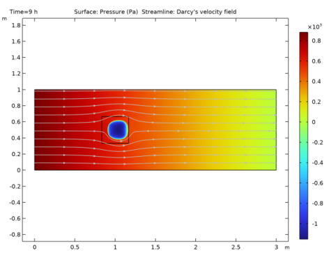
The simulation is run for 56 hours which is the time until the frozen inclusion is completely melted and the cooler temperatures have been convected out of the channel. However, it is also interesting to display the effect of the molten inclusion on the pressure and temperature distribution; Figure 2 shows the pressure distribution after 9 hours of simulated time when there is still some ice present. As gravity has been neglected, only the pressure effects of the ice inclusion are shown.]

Figure 2: Pressure distribution after 9 hours when there is still some ice present in the model domain.

The temperature field is shown at the same time (after 9 hours) in Figure 3 and the liquid water saturation in Figure 4. Both figures indicate the ice inclusion and its influence on the temperature field. The low temperatures are convected in the downstream part of the domain.

Figure 3: Surface plot showing the temperature distribution after 9 hours.

Figure 4: Surface plot showing the liquid water saturation after 9 hours. Effectively the areas with liquid water appear in blue whereas the areas of ice appear in white.

The plots below have been used as performance measures in the INTERFROST benchmark, and therefore are also included here:

The evolution of the minimum of the simulated temperature field as a function of time is shown in Figure 5..

Figure 5: The minimum temperature in the model domain as a function of time.

Figure 6 shows the time evolution of the total heat flux exiting the system at the downstream boundary.

Figure 6: Total heat flux exiting the system via the outflow boundary as a function of time.

Figure 7 displays the evolution of the total liquid water volume in the domain as a function of time.

Figure 7: Total liquid water volume in the domain as a function of time.

Notes About the COMSOL Implementation

A residual liquid phase is present in soils even for temperatures significantly below 0°C. To make sure that this residual water is not subject to phase change in the model and that it is not convected, it is considered as a second immobile solid (in addition to the solid matrix). According to Ref. 1, the residual saturation Sw, res is set to 0.05.

References

1. C. Grenier and others, “Groundwater flow and heat transport for systems undergoing freeze-thaw: Intercomparison of numerical simulators for 2D test cases,” Advances in Water Resources, vol. 114, pp. 196–218, 2018.

2. https://wiki.lsce.ipsl.fr/interfrost/doku.php?id=test_cases:five

Subsurface_Flow_Module/Heat_Transfer/frozen_inclusion

Modeling Instructions

From the menu, choose .

New

In the window, click

Model Wizard

In the window, click

In the tree, select .

Right-click and choose .

In the tree, select .

Right-click and choose .

Click

In the tree, select .

Click

Global Definitions

Parameters 1

In the window, under click .

The parameters defining the material properties of the solid matrix, water, and ice have to be declared. They are available in a file and you can import them as follows:

In the window for , locate the section.

Click

Browse to the model’s Application Libraries folder and double-click the file frozen_inclusion_parameters.txt.

Geometry 1

Now, the model domain is drawn as two rectangles, one representing the porous domain, the other the frozen inclusion within the porous domain. Create the geometry as follows and note that due to symmetry only half of the model domain is drawn.

Rectangle 1 (r1)

In the toolbar, click

In the window for , locate the section.

In the text field, type 3.

In the text field, type 0.5.

Rectangle 2 (r2)

In the toolbar, click

In the window for , locate the section.

In the text field, type 0.333.

In the text field, type 0.333/2.

Locate the section. From the list, choose .

In the text field, type 1.

In the text field, type 0.5-0.333/4.

In the toolbar, click

Materials

Define the materials in the next step. Introduce them as empty material nodes, first. As soon as the physics has been defined, the material node menu will show you which properties are needed for the simulation. You can then just fill in the values defined in the list.

Solid Matrix

In the window, under right-click and choose .

In the window for , type Solid Matrix in the text field.

Water

Right-click and choose .

In the window for , type Water in the text field.

Ice

Right-click and choose .

In the window for , type Ice in the text field.

Porous Material 1 (pmat1)

Right-click and choose .

In the window for , locate the section.

From the list, choose .

Locate the section. Click

Fluid 1 (pmat1.fluid1)

In the window, click .

In the window for , locate the section.

From the list, choose .

Solid 1 (pmat1.solid1)

In the window, click .

In the window for , locate the section.

From the list, choose .

In the θs text field, type 1-epsilon_p.

Immobile Fluid 1 (pmat1.imfluid1)

In the window, right-click and choose .

In the window for , locate the section.

From the list, choose .

In the θimf text field, type epsilon_p*Sw_res.

Heat Transfer in Porous Media (ht)

Continue with setting up the physics. Since some heat transfer variables are needed to define the saturation variables as explained in the Model Definition section, start with Heat Transfer in Porous Media (ht).

In the window, under click .

In the window for , locate the section.

In the Tref text field, type T_initial_w.

Porous Matrix 1

In the window, under click .

In the window for , locate the section.

From the list, choose , because the properties of a pure solid material are given.

With the following steps you define the residual liquid water volume as product of porosity and predefined residual water saturation.

Porous Medium 1

In the window, click .

Immobile Fluids 1

In the toolbar, click

and choose .

Fluid 1

In the window, click .

In the window for , locate the section.

From the pA list, choose .

Locate the section. From the u list, choose .

Phase Change Material 1

In the toolbar, click

and choose .

Phase Change Material 1

In the window, expand the node, then click .

In the window for , click to expand the section.

Inflate the sketch to visualize which material you have to choose for which temperatures. In this case, material 1 should be ice, material 2 water. You will use the function θ2 later when you define the water saturation as a function of phase change.

Locate the section. In the Tpc,1 → 2 text field, type T_pc.

In the ΔT1 → 2 text field, type 1[K].

In the L1 → 2 text field, type L.

Locate the section. From the list, choose .

Initial Values 1

In the window, under click .

In the window for , locate the section.

In the T text field, type T_initial_w.

Initial Values 2

In the toolbar, click

and choose .

Select Domain 2 only.

In the window for , locate the section.

In the T text field, type T_initial_i.

Temperature 1

In the toolbar, click

and choose .

Select Boundary 1 only.

In the window for , locate the section.

In the T0 text field, type T_initial_w.

Outflow 1

In the toolbar, click

and choose .

Select Boundary 9 only.

Symmetry 1

In the toolbar, click

and choose .

Select Boundaries 3, 6, and 8 only.

Definitions (comp1)

For Darcy’s Law the water saturation and the permeability have to be defined as temperature-dependent variables. More precisely they depend on θ2 which is the fraction of water due to phase change.

Variables 1

In the window, expand the node.

Right-click and choose .

In the window for , locate the section.

In the table, enter the following settings:


Name	Expression	Unit	Description
Sw	Sw_res+(1-Sw_res)*ht.theta2		Water saturation
kr	max(10^(-Omegaepsilon_p(1-Sw)),1e-6)		Relative permeability
kappa_w	k_int*kr	m²	Permeability

Darcy’s Law (dl)

In the window, under click .

In the window for , click to expand the section.

From the list, choose .

Change the shape function to linear to reduce the computational time and increase numerical stability.

Porous Medium 1

In the window, under click .

In the window for , locate the section.

From the list, choose . In the Sp text field, type Sw*epsilon_p*beta.

Porous Matrix 1

In the window, click .

In the window for , locate the section.

From the εp list, choose . In the associated text field, type epsilon_p*Sw.

Mass Source 1

In the toolbar, click

and choose .

The mass source accounts for the addition of water during melting as described in the Model Definition section.

In the window for , locate the section.

From the list, choose .

Locate the section. In the Qm text field, type dl.epsilon*(rho_i-rho_w)*d(Sw,t). Remember that dl.epsilon was defined as epsilon_p*Sw to represent only the pore space that is filled with water.

The flow is driven by an imposed gradient of the hydraulic head. This is defined as a parameter and could be varied in a parametric sweep in future simulations (as it was done in the INTERFROST project, see References).

Hydraulic Head 1

In the toolbar, click

and choose .

Select Boundary 1 only.

In the window for , locate the section.

In the H0 text field, type delta_H_dLx*3[m].

Hydraulic Head 2

In the toolbar, click

and choose .

Select Boundary 9 only.

Symmetry 1

In the toolbar, click

and choose .

Select Boundaries 3, 6, and 8 only.

Materials

Having defined the physics, now fill in the empty expressions in the node.

Porous Material 1 (pmat1)

In the window, under click .

In the window for , locate the section.

In the table, enter the following settings:


Property	Variable	Value	Unit	Property group
Permeability	kappa_iso ; kappaii = kappa_iso, kappaij = 0	kappa_w	m²	Basic

Solid Matrix (mat1)

In the window, click .

In the window for , locate the section.

In the table, enter the following settings:


Property	Variable	Value	Unit	Property group
Density	rho	rho_s	kg/m³	Basic
Thermal conductivity	k_iso ; kii = k_iso, kij = 0	lambda_s	W/(m·K)	Basic
Heat capacity at constant pressure	Cp	Cs	J/(kg·K)	Basic

Water (mat2)

In the window, click .

In the window for , locate the section.

In the table, enter the following settings:


Property	Variable	Value	Unit	Property group
Density	rho	rho_w	kg/m³	Basic
Dynamic viscosity	mu	mu_w	Pa·s	Basic
Thermal conductivity	k_iso ; kii = k_iso, kij = 0	lambda_w	W/(m·K)	Basic
Heat capacity at constant pressure	Cp	Cw	J/(kg·K)	Basic

Ice (mat3)

In the window, click .

In the window for , locate the section.

In the table, enter the following settings:


Property	Variable	Value	Unit	Property group
Thermal conductivity	k_iso ; kii = k_iso, kij = 0	lambda_i	W/(m·K)	Basic
Density	rho	rho_i	kg/m³	Basic
Heat capacity at constant pressure	Cp	Ci	J/(kg·K)	Basic