PDF

Forchheimer Flow
Introduction
This is a tutorial of the coupling between flow of a fluid in an open channel and a porous block attached to one of the channel walls. The flow is described by the Navier-Stokes equation in the free region and a Forchheimer-corrected version of the Brinkman equations in the porous region.
Figure 1: Depiction of the modeling geometry and domain. The 3D geometry can be reduced to a 2D representation assuming that changes through the thickness are negligible.
The coupling of free media flow with porous media flow is common in the fields of earth science and chemical engineering. Perhaps the most frequent way to deal with coupled free and porous media flow is to incorporate Darcy’s law adjacent to Navier-Stokes because it is usually numerically easy to solve. However, this approach does not account for viscous effects arising from the free media flow, which may still be important in the region close to the free-porous structure interface. Depending on the pore size and pore distribution, but also the fluid’s properties, it can therefore be an oversimplification to employ Darcy’s law. The Brinkman equations account for momentum transport by macroscopic viscous effects as well as pressure gradients (stemming from microscopic shear effects inside each pore channel) and can be considered an extension of Darcy’s Law.
Still, the Brinkman equations assume laminar flow. Looking at processes in relatively open structures, like gas flow through packed beds, there is also a turbulent contribution to the resistance to flow. In those cases, an additional term accounts for the turbulent contribution to the resistance to flow in the porous domain. The Forchheimer equation (also accredited to Ergun) is widely used to predict pressure drops in packed beds. This equation can generally be written as
The left-hand side is the pressure drop per unit length of traveled distance through the bed. The first term on the right-hand side represents the Blake-Kozeny equation for laminar flow. The pressure drop depends linearly on the average linear velocity u for laminar flow, corresponding to Darcy flow. The second term is from the purely turbulent Burke-Plummer equation where the pressure drop is proportional to the square of the velocity. Description of an intermediate flow, where both the laminar and turbulent effects are important, requires the two-term Forchheimer equation. The coefficients α1 and α2 are functions of porosity, viscosity, average pore diameter, and fluid density.
Model Definition
Figure 2 below shows the example domain and notations for the boundary conditions.
Figure 2: Modeled domain and boundary notations. Flow enters at the bottom and leaves at the top. The region of porous structure is not as long as the free channel.
Flow in the free channel is described by the stationary, incompressible Navier-Stokes equations:
(1)
where μ denotes the dynamic viscosity (Pa·s), u refers to the velocity in the open channel (m/s), ρ is the fluid’s density (kg/m3), and p is the pressure (Pa). In the porous domain, the Brinkman equations with Forchheimer correction describe the flow:
(2)
Here κ denotes the permeability of the porous medium (m2), εp is the porosity (dimensionless), and the dimensionless friction coefficient is (Ref. 1)
As Equation 1 and Equation 2 reveal, the momentum transport equations are closely related. The term on the left-hand side of the Navier-Stokes formulation corresponds to momentum transferred by convection in free flow. The Brinkman formulation replaces this term by a contribution associated with the drag force experienced by the fluid flowing through a porous medium. In addition, the last term in the right-hand side of Equation 2 presents the Forchheimer correction for turbulent drag contributions.
In COMSOL Multiphysics, it is easy to set up and solve such a coupled flow regime. The implementation of the extra drag is done with a Forchheimer coefficient (kg/m4) equal to
At the flow inlet a normal inflow velocity u=-U0n is defined. At the flow outlet the fluid can leave the domain. The outlet boundary condition with the pressure option selected sets the normal stress component equal to the pressure at the outlet. The tangential stress component vanishes. All other boundaries are defined as walls with a no slip condition u=0.
The following table lists the input data for the example:
μ
10-3 kg/(m·s)
ρ
κ
10-7 m2
v0
Results and Discussion
Figure 3 shows the velocity field in the open channel and porous structure. The plot reveals that there are slight disturbances in the velocity at the porous wall, which suggests momentum transport by viscous effects.
Figure 3: Velocity field without Forchheimer correction (left) and with Forchheimer correction (right).
Figure 4 contains a cross-sectional velocity plot. It shows that without the Forchheimer correction, the resistance to flow is underestimated in the porous domain. The added correction gives a solution with slower flow in the porous domain and a faster flow in the free domain, due to incompressibility.
Figure 4: Cross section of the velocity field (velocity magnitude) in the middle of the modeling domain with and without the Forchheimer correction.
Further postprocessing would show that the shear rate perpendicular to the flow is also continuous. This implies that there is significant viscous momentum transfer across the interface and into the porous material, a transport that is not accounted for by Darcy’s law.
Notes About the COMSOL Implementation
To implement the Forchheimer pressure drop relation in a differential equation framework, this example uses an approach suggested in Ref. 1 in which the Brinkman momentum balance is amended with a Forchheimer term. The system studied in this example is that of a 2D cross section of a rectangular channel with a porous layer attached to one of its walls. Flow enters the volume with a uniform velocity profile and develops throughout the length of the channel.
Reference
1. A. Amiri and K. Vafai, “Transient Analysis of Incompressible Flow Through a Packed Bed,” Int. J. Heat and Mass Transfer, vol. 41, pp. 4259–4279, 1998.
Application Library path: Subsurface_Flow_Module/Fluid_Flow/forchheimer_flow
Modeling Instructions
From the File menu, choose New.
New
In the New window, click  Model Wizard.
Model Wizard
1
In the Model Wizard window, click  2D.
2
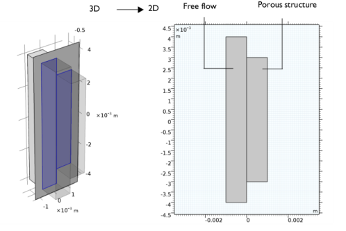
In the Select Physics tree, select Fluid Flow>Porous Media and Subsurface Flow>Free and Porous Media Flow (fp).
3
4
Click  Study.
5
In the Select Study tree, select General Studies>Stationary.
6
Geometry 1
Rectangle 1 (r1)
1
In the Geometry toolbar, click  Rectangle.
2
In the Settings window for Rectangle, locate the Size and Shape section.
3
In the Width text field, type 1e-3.
4
In the Height text field, type 6e-3.
5
Locate the Position section. In the y text field, type -3e-3.
Rectangle 2 (r2)
1
In the Geometry toolbar, click  Rectangle.
2
In the Settings window for Rectangle, locate the Size and Shape section.
3
In the Width text field, type 1e-3.
4
In the Height text field, type 8e-3.
5
Locate the Position section. In the x text field, type -1e-3.
6
In the y text field, type -4e-3.
7
In the Geometry toolbar, click  Build All.
Global Definitions
Parameters 1
1
In the Model Builder window, under Global Definitions click Parameters 1.
2
In the Settings window for Parameters, locate the Parameters section.
3
Free and Porous Media Flow (fp)
Porous Medium 1
1
In the Model Builder window, under Component 1 (comp1) right-click Free and Porous Media Flow (fp) and choose Porous Medium.
2
Materials
Fluid
1
In the Model Builder window, under Component 1 (comp1) right-click Materials and choose Blank Material.
2
In the Settings window for Material, type Fluid in the Label text field.
3
Locate the Material Contents section. In the table, enter the following settings:
Porous Material 1 (pmat1)
1
Right-click Materials and choose More Materials>Porous Material.
2
3
In the Settings window for Porous Material, locate the Porosity section.
4
In the εp text field, type eps_p.
5
Locate the Homogenized Properties section. In the table, enter the following settings:
6
Locate the Phase-Specific Properties section. Click  Add Required Phase Nodes.
Fluid 1 (pmat1.fluid1)
1
In the Model Builder window, click Fluid 1 (pmat1.fluid1).
2
In the Settings window for Fluid, locate the Fluid Properties section.
3
From the Material list, choose Fluid (mat1).
Free and Porous Media Flow (fp)
Porous Medium 1
1
In the Model Builder window, under Component 1 (comp1)>Free and Porous Media Flow (fp) click Porous Medium 1.
2
In the Settings window for Porous Medium, locate the Porous Medium section.
3
From the Flow model list, choose Non-Darcian flow.
Porous Matrix 1
1
In the Model Builder window, expand the Porous Medium 1 node, then click Porous Matrix 1.
2
In the Settings window for Porous Matrix, locate the Matrix Properties section.
3
In the cF text field, type fs*Cf.
Inlet 1
1
In the Physics toolbar, click  Boundaries and choose Inlet.
2
3
In the Settings window for Inlet, locate the Velocity section.
4
In the U0 text field, type v0.
Outlet 1
1
In the Physics toolbar, click  Boundaries and choose Outlet.
2
Mesh 1
1
In the Model Builder window, under Component 1 (comp1) click Mesh 1.
2
In the Settings window for Mesh, locate the Physics-Controlled Mesh section.
3
From the Element size list, choose Fine.
4
Click  Build All.
The physics-controlled mesh automatically generates a boundary layer mesh at the walls where steep velocity gradients are expected.
Study 1
Step 1: Stationary
1
In the Model Builder window, under Study 1 click Step 1: Stationary.
2
In the Settings window for Stationary, click to expand the Study Extensions section.
3
Select the Auxiliary sweep check box.
4
5
6
In the Home toolbar, click  Compute.
Results
Velocity (fp)
Visualize the velocity fields as in Figure 3.
1
In the Settings window for 2D Plot Group, locate the Data section.
2
From the Parameter value (fs) list, choose 0.
Streamline 1
1
Right-click Velocity (fp) and choose Streamline.
2
In the Settings window for Streamline, locate the Streamline Positioning section.
3
In the Number text field, type 8.
4
5
Locate the Coloring and Style section. Find the Point style subsection. From the Type list, choose Arrow.
6
From the Arrow distribution list, choose Equal time.
7
From the Color list, choose White.
Create a plot for the solution including the Forchheimer drag (fs=1) next to the plot as follows.
Velocity (fp)
1
In the Model Builder window, click Velocity (fp).
2
In the Settings window for 2D Plot Group, click to expand the Title section.
3
From the Title type list, choose Manual.
4
Clear the Parameter indicator text field.
5
Click to expand the Plot Array section. Select the Enable check box.
Streamline 1
1
In the Model Builder window, click Streamline 1.
2
In the Settings window for Streamline, click to expand the Plot Array section.
3
Select the Manual indexing check box.
Streamline 1, Surface
1
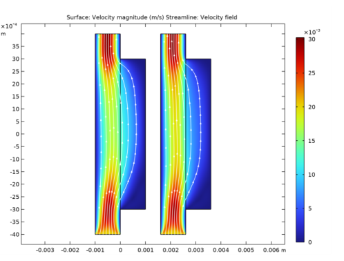
In the Model Builder window, under Results>Velocity (fp), Ctrl-click to select Surface and Streamline 1.
2
Surface 2
1
In the Settings window for Surface, locate the Data section.
2
From the Dataset list, choose Study 1/Solution 1 (sol1).
3
Click to expand the Inherit Style section. From the Plot list, choose Surface.
Streamline 2
1
In the Model Builder window, click Streamline 2.
2
In the Settings window for Streamline, locate the Data section.
3
From the Dataset list, choose Study 1/Solution 1 (sol1).
4
Locate the Plot Array section. In the Index text field, type 1.
5
Click to expand the Inherit Style section. In the Velocity (fp) toolbar, click  Plot.
6
Click the  Zoom Extents button in the Graphics toolbar.
Create the plot from Figure 4.
Cut Line 2D 1
1
In the Results toolbar, click  Cut Line 2D.
2
In the Settings window for Cut Line 2D, locate the Line Data section.
3
In row Point 1, set x to -1e3.
4
In row Point 2, set x to 1e3.
Velocity magnitude
1
In the Results toolbar, click  1D Plot Group.
2
In the Settings window for 1D Plot Group, type Velocity magnitude in the Label text field.
Line Graph 1
1
Right-click Velocity magnitude and choose Line Graph.
2
In the Settings window for Line Graph, locate the Data section.
3
From the Dataset list, choose Cut Line 2D 1.
4
In the Velocity magnitude toolbar, click  Plot.
5
Click to expand the Coloring and Style section. Find the Line markers subsection. From the Marker list, choose Cycle.
6
Click to expand the Legends section. Select the Show legends check box.
7
Find the Prefix and suffix subsection. Click thebutton. From the menu, choose Global definitions>Parameters>fs - Switch for Forchheimer terms.
8
In the Prefix text field, type fs=.
9
In the Velocity magnitude toolbar, click  Plot.